Lot’s of data. Lot’s of signal claims. Lot’s of excitement. Lot’s of work.
List of upcoming experiments
LHAASO ~2021
CTA ~2025
AMEGO
XRISM ~2022
SKA ~2025
\(\newcommand{\indep}{\perp\!\!\!\perp}\)
A typical day in indirect DM search land
Optimist: I took your gamma-ray data, subtracted a model for astrophysical emission, and what is left looks pretty much like a signal from self-annihilating WIMPs.
Pessimist: The astrophysical emission model you are using is full of systematic uncertainties. You cannot conclude anything from looking at data-model residuals.
Optimist: Look at my 100 pages appendix where I account for all uncertainties and show that my findings are robust.
Pessimist: I am not going to read your appendix. Every week there is another dark matter “discovery”, none of them have been proven right.
Optimist: This time it is real. And history will prove me right.
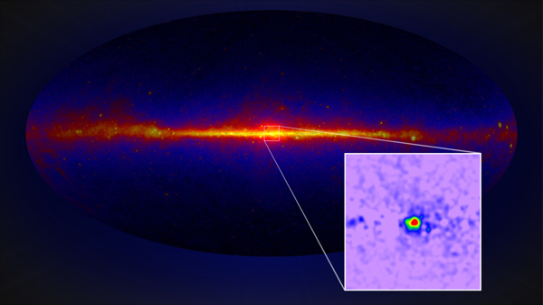
The Fermi Galactic center GeV excess is a candidate for a dark matter signal, since Goodenough & Hooper 2008, here from Fermi coll. 2017.
Example: The Fermi GeV excess
Point sources (millisecond pulsars) vs dark matter.
There are dozens of papers on the topic, many in favor of a dark matter interpretation, and many in favor of a astrophysical explanation.
Example: The Fermi GeV excess
One of the most recent papers, List+ 2006.12504, finds supporting evidence for a point source interpretation.
Why can’t we just agree?
It seems simple:
Step 1: Describe what we know/do not know about signals and backgrounds.
Step 2: Compare with data.
Step 3: Draw conclusions.
This is the outline of this lecture.
Step 1. How to describe what we know and do not know about signals and backgrounds.
Summarize/describe what we know: rest of this PhD school.
How to describe what we do not know: here.
Caveat: I will here focus on “known unknowns”, things that we are in principle aware of and can describe. There is also the problem of unknown unknowns (related to the field of anomaly detection). However, in many cases there are already so many unaddressed problems with known unknowns that it is a good idea to focus on that first.
From coin flips to normal distribution
Many binary choices can lead to the normal distribution
Random variables & probabilities
A random variable is some aspect of the world that is intrinsically uncertain.
Random variables \(X\) have domains (sample space, \(\Omega_X\))
Discrete domains (object classes, number of objects, …)
Side remark: Random variables are often written in capital letters (\(X\), \(Y\), …), actual outcome/observation/measurement often in lower case letters (\(x\), \(y\), …)
Examples for probability distributions
The basics of probability distributions
Probabilities for all possible measurment outcomes sum/integrate to one, \[
\sum_{x \in \Omega_X} p(x) = 1\;,\quad \text{or}\quad
\int_{\Omega_X} dx\, p(x) = 1\;.
\]
Joint distributions assign probabilities to a combination of random variables, \((x, y, \dots)\), and sum to one. \[\sum_{x \in \Omega_x, y \in \Omega_y, \dots} P(x, y, \dots)=1\]
Given some joint distribution, we are often only interested in the distribution of a single random variable. We can obtain it by marginalization. \[
p(x) = \sum_{y\in \Omega_y} p(x, y)
\]
\(t\)
\(p(t)\)
COLD
0.4
WARM
0.6
\(t\)
\(w\)
\(p(t, w)\)
COLD
RAIN
0.2
WARM
RAIN
0.1
COLD
SUN
0.2
WARM
SUN
0.5
\(w\)
\(p(w)\)
RAIN
0.3
SUN
0.7
Frequentist interpretation of probability
When repeating the same experiment multiple times, the number of occurrences of a specific event, relative to the total number of experiments, would tend towards the probability. \[ \lim_{N\to\infty} \frac{n_i}{N} \to p_i \]
For a finite number of possibe outcomes, this can be represented as a discrete \(P[X = x] = p_X(x) = p_x\) distribution table.
Bayesian interpretation of probability
Proposition A = “Next Sunday there will be rain.”
\(P(A)=1\): Proposition is true
\(P(A)=0\): The proposition is false
\(P(A)=\frac12\): The position is equally likely to be true or false
Bayesian probabilities allow statements about the plausibility (or our subjective belief) of propositions, independently of whether experiments can be repeated or not.
Bayesian probabilities can be thought of extensions of binary logic to incorporate reasoning about uncertainty.
Bayes rule allows you to update your prior belief given new observational data.
Probabilistic models
At a very fundamental level, all our uncertaintiy about the possible experimental outcomes of a measurement are described by a single high-dimensional joint probability distribution, \[
p(x_1, x_2, x_3, \dots, x_N)\;.
\]
\(x_1, \dots, x_N\): List of everything uncertain (number of detected photons in a image pixel, value of the cosmological constant, Hubble rate, mass of the electron, size of effective area, position of a gamma-ray source, luminosity of a radio source, …)
Conditional probabilities are relating joint and marginal probability\[P(x| y) \equiv \frac{P(x, y)}{P(y)}\]
Example: Which fraction of the area is red, blue, red+blue or none?
Area = Probability
Total area = 1
The chain rule
A consequence of the definition of conditional probabilities is the chain rule. We can always decompose a joint distribution like \[
p(x_1, x_2) = p(x_1)p(x_2|x_1)
\]\[
p(x_1, x_2, x_3) = p(x_1)p(x_2, x_3|x_1) = p(x_1)p(x_2|x_1) p(x_3|x_1, x_2)
\]\[
\dots
\]\[
\begin{multline}
p(x_1, x_2, x_3, \dots, x_n) = \\p(x_1) p(x_2|x_1) p(x_3|x_1, x_2) \dots p(x_n| x_1, x_2, \dots, x_{n-1})\;.
\end{multline}
\]
This can be visualized with a directed acyclic graph (DAG)
Probabilistic independence
Two random variables \(x\) and \(y\) are independent if \[\forall x, y: P(x, y) = P(x)P(y) \quad \Leftrightarrow \quad
\forall x, y: P(x|y) = P(x)\]
One can write \(X \indep Y\), or say “the joint distribution factors into two simpler distributions”.
If two variables are probabilistically independent, measuring one does not imply anything for the other variable.
Conditional independence
In reality, things are seldomly completely independent
The best we can hope for is conditional independence.
This means: given \(Z\), \(X\) and \(Y\) are independent: \(X\indep Y|Z\)
Mathematically, this means (all three expressions are equivalent) \[\forall x, y, z: P(x, y|z) = P(x|z) P (y|z)\]\[\forall x, y, z: P(x|y, z) = P(x|z)\]\[\forall x, y, z: P(y|x, z) = P(y|z)\]
Conditional independence is a basic but robust framework for reasoning about an uncertain environment. Not that in general we will still have that \(p(x, y) \neq p(x)p(y)\).
This motivates Bayes nets, which enable us to reason about the correlation structure of probabilistic models.
For a given DM hypothesis \(\mathcal{H}\), our knowledge about the data \(\mathbf x\), as well as the underlying interesting (\(\boldsymbol \nu\)) and uninteresting (\(\boldsymbol \eta\)) physics can be in principle encoded in a Bayesian net.
A simple toy model: Diffuse emission + point sources
Data
One energy range
50 x 50 spatial pixels (Galactic longitude vs and latitude)
Two diffuse emission components
Galactic disk
Isotropic background
One point source population
Power-law with cutoffs
Isotropical source distribution
We nelgect complications due to
Angular resolution
Uncertainties in the emission components
1. The diffuse emission component
We have a simple three-parameter model for the diffuse emission \[
f_\text{diff}(\ell, b) = \theta_\text{iso} + \theta_\text{dn}\exp\left(-\frac12 \frac{b^2}{\theta_\text{dw}^2}\right)
\]
Expected number of photons in pixel \(i\) (defined by \(\Omega_i\)) \[
\lambda_i = \int_{\Delta\Omega_i} d\ell\, db \; f_\text{diff}(\ell, b) \cdot \mathcal{E}
\]
The number of measured photons is then distributed like \[
c_i \sim \text{Pois}(\lambda_i)
\]
2. The point source component
We have \(N_\text{psc}\geq 0\) number of sources in our anlaysis region.
Their fluxes are distributed like \[
p_\text{psc}(F) =
\left\{
\begin{matrix}
\frac{\gamma-1}{F_\text{min}^{1-\gamma} - F_\text{max}^{1-\gamma}}F^{-\gamma} & \text{for}\quad F_\text{min} \leq F \leq F_\text{max}\\
0 & \text{otherwise}
\end{matrix}
\right.
\;,
\] where \(\gamma\) is the index of the flux distribution function. We assume \(\gamma > 1\).
A random draw of the source population works as follows
Sample random source positions \(\ell_k, b_k \sim \text{Unif}(-1, 1)\), for \(k = 1, \dots, N_\text{psc}\)
Then the gamma-ray emission map can be written as \[
f_\text{psc}(\ell, b) = \sum_{k=1}^{N_\text{psc}} F_k \delta_D(\ell - \ell_k) \delta_D(b - b_k)
\]
If source \(k\) is contained in pixel \(i\), the expected number of additional photon counts is given by \(\lambda_i = \mathcal{E} F_k\).
Our model has \(5 + N_\text{psc}\times 3\) random parameters (typically thousands)
The number of parameters of the model is itself uncertain.
The model is far simpler than any real simulation of gamma-ray data, yet complex enough to highlight the challenges of statistical analysis.
The “inverse problem”: Given some observation, how can we infer a plausible range of model parameters that is consistent with the observation?
How to infer diffuse emission parameters?
Let’s assume we are interested in the posterior for the diffuse parameters. Easy-peasy. We write down Bayes theorem. \[
p(\theta_\text{dn},
\theta_\text{dw},
\theta_\text{iso}
|\mathbf c) =
\frac{p(\mathbf c| \theta_\text{dn}, \theta_\text{dw}, \theta_\text{iso}) p(\theta_\text{dn})p(\theta_\text{dw})p(\theta_\text{iso})}{p(\mathbf c)}
\]
Here, we made use of the marginal likelihood, where we marginalize out the point source parameters (since we are not interested in them) \[
\begin{multline}
p(\mathbf c|\theta_\text{dn}, \theta_\text{dw}, \theta_\text{iso}) = \sum_{N_\text{psc}=0}^\infty p(N_\text{psc}) \int
d\gamma
\left(\prod_{k=1}^{N_\text{psc}}\, d\ell_k\, db_k\, dF_k\,
p_\text{psc}(F_k|\gamma)\, p(\ell_k, b_k) \right) \times
\\
\times\left( \prod_{i=1}^{N_\text{pix}}p(c_i| \lambda_i (\theta_\text{iso}, \theta_\text{dn}, \theta_\text{dw}, \mathbf F, \mathbf b, \boldsymbol \ell)) \right)
p(\gamma)
\end{multline}
\]
This integral is extremely hard to solve or approximate in general, and is usually not done. Instead, one typically masks sources, ignores them, or tries to model them individually source-by-source. In all cases, we have to make simplifying assumptions.
Let’s assume we solved the point source parameter problem (e.g. by masking all pixels of the image that seem to contain a source).
In that case the model is relatively simple, \[
p(\mathbf c | \theta) = \prod_{i=1}^{N_\text{pix}}\text{Pois}(c_i|\lambda_i(\theta))
\] where \[
\lambda_i = \mathcal{E} \Delta\Omega \left(\theta_\text{iso} + \theta_\text{dn} \exp\left(-\frac12 \frac{b_i^2}{\theta_{dw}^2}\right) \right)
\]
This is a 3-dim problem that we could feed into some sampler, and obtain posteriors for the parameters.
Still, we will have unresolved sources that will contribute in this case to the emission. We have to estimate and correct for their effect by hand.
Estimating the expected uncertainties
We can use Fisher forecasting techniques to estimate the expected parameter uncertainties.
The Fisher information matrix is given by \[
\mathcal{I}_{nm} = \sum_i \mathbb{E}_{c_i \sim p(c_i|\lambda_i(\boldsymbol \theta))} \left[
\left(\frac{\partial}{\partial \theta_n} \ln p(c_i|\lambda_i(\boldsymbol\theta))\right)
\left(\frac{\partial}{\partial \theta_m} \ln p(c_i|\lambda_i(\boldsymbol\theta))\right)
\right]
= \sum_i \
\frac{\partial \lambda_i}{\partial \theta_n} \frac{1}{\lambda_i(\boldsymbol\theta)} \frac{\partial \lambda_i}{\partial \theta_m}\;,
\] where the last step is valid for Poisson likelihoods. Remember that the poisson distribution is given by \[
\text{Pois}(c|\lambda) = \frac{\lambda^c e^{-\lambda}}{c!}\;.
\]
The inverse of the Fisher matrix provides an estimate of the covariance matrix \[
\Sigma = \mathcal{I}^{-1}
\]
How to infer point source parameters?
Easy-peasy. We write down Bayes theorem. \[
p(\gamma, N_\text{psc}|\mathbf c) =
\frac{p(\mathbf c| \gamma, N_\text{psc}) p(\gamma)p(N_\text{psc})}{p(\mathbf c)}
\]
Here, we made use of the marginal likelihood, where we marginalize out individual point sources and diffuse emission parameters (since we are not interested in them) \[
\begin{multline}
p(\mathbf c|\gamma, N_\text{psc}) = \int
d\theta_\text{dn}\,
d\theta_\text{dw}\,
d\theta_\text{iso}\,
\left(\prod_{k=1}^{N_\text{psc}}\, d\ell_k\, db_k\, dF_k\,
p_\text{psc}(F_k|\gamma)\, p(\ell_k, b_k) \right) \times
\\
\times\left( \prod_{i=1}^{N_\text{pix}}p(c_i| \lambda_i (\theta_\text{iso}, \theta_\text{dn}, \theta_\text{dw}, \mathbf F, \mathbf b, \boldsymbol \ell)) \right)
p(\theta_\text{dn})
p(\theta_\text{dw})
p(\theta_\text{iso})
\end{multline}
\]
Again, this integral is extremely hard to solve.
Let’s assume that diffuse backgrounds are known. In that case, the photon counts in each pixel become conditionally independent given the population parameters.
One can find (via MC simulations, or clever analytic calculations) an effective marginal likelihood of the form \[
p(\mathbf c|\gamma, N_\text{psc}) = \prod_{i=1}^{N_\text{pix}}p_\text{eff}(c_i| \lambda_i (\gamma, N_\text{psc}))
\]
Once we simulated or calculated \(p_\text{eff}\), we can again use simple MCMC techniques etc to explore the 2-dim posterior.
However, this approach neglects any uncertainties in the diffuse emission component.
Lessons from the toy model
In order to study diffuse emission parameters with template regression, we had to neglect uncertainties in point sources.
In order to study point source population parameters with 1-point PDF, we had to neglect uncertainties in diffuse emission.
And this was a simple toy model, which neglected:
Multiple diffuse components
Uncertainties of diffuse emission templates
Energy dependence
Spatial variations in point source distributions
Point source associations
Multiple source populations
Taking into account all model uncertatinies at the same time is in general really hard, not (only) from the modeling perspective, but from the inference perspective.
So far we considered the logistic unit \(h=\sigma\left(\mathbf{w}^T \mathbf{x} + b\right)\), where \(h \in \mathbb{R}\), \(\mathbf{x} \in \mathbb{R}^p\), \(\mathbf{w} \in \mathbb{R}^p\) and \(b \in \mathbb{R}\).
These units can be composed in parallel to form a layer with \(q\) outputs: \[\mathbf{h} = \sigma(\mathbf{W}^T \mathbf{x} + \mathbf{b})\] where \(\mathbf{h} \in \mathbb{R}^q\), \(\mathbf{x} \in \mathbb{R}^p\), \(\mathbf{W} \in \mathbb{R}^{p\times q}\), \(b \in \mathbb{R}^q\) and where \(\sigma(\cdot)\) is upgraded to the element-wise sigmoid function.
Similarly, layers can be composed in series, such that: \[\begin{aligned}
\mathbf{h}_0 &= \mathbf{x} \\
\mathbf{h}_1 &= \sigma(\mathbf{W}_1^T \mathbf{h}_0 + \mathbf{b}_1) \\
... \\
\mathbf{h}_L &= \sigma(\mathbf{W}_L^T \mathbf{h}_{L-1} + \mathbf{b}_L) \\
f(\mathbf{x}; \theta) = \hat{y} &= \mathbf{h}_L
\end{aligned}\] where \(\theta\) denotes the model parameters \(\{ \mathbf{W}_k, \mathbf{b}_k, ... | k=1, ..., L\}\).
This model is the multi-layer perceptron, also known as the fully connected feedforward network.
As a warm up, let us minimize the loss function \[
L(M) = \int dx\, p(x) (M - x)^2
\] w.r.t. variable \(M \in \mathbb{R}\). Setting \(dL/dM = 0\) yields \(M = \mathbb{E}_{x\sim p(x)}[x]\).
Now let us consider minimizing the function \(M(y)\), with the loss functional given by \[
L[M] = \int dx\, p(x, y) (M(y) - x)^2
\] Minimization (setting \(\delta L/\delta M(y)= 0\) for all \(y\)) yields now \(M(y) = \mathbb{E}_{x \sim p(x|y)} [x]\).
Stochastic gradient descent
We can approximate the integral by summing over a large number of samples \(x_i \sim p(x)\) from the target distribution \[
L[\phi] = \int dx\, p(x) \ell_\phi(x) \approx \frac{1}{N} \sum_{i=1}^N \ell_\phi(x_i)
\]
Use stochastic gradient descent to optimize - instead of using all \(N\) training samples, we only use constantly changing subsets \(\mathcal{B}\)\[
\nabla_\phi L[\phi] \approx \frac{1}{|\mathcal{B}|} \sum_{i\in \mathcal{B}} \nabla_\phi \ell_\phi(x_i)
\]
Gradient Descent
To minimize the error function \(E(\theta)\) defined over model parameters \(\theta\) (e.g. \(\mathbf{w}\) and \(b\)), the simplest gradient method of gradient descent uses local linear information to iteratively move towards a local minimum. The algorithm must be initialized with an initial value of parameters \(\theta_0\). A first order approximation to \(E(\theta)\) around \(\theta_0\) can be given as
We can minimize the approximation \(\hat{E}({\theta }_0)\) in the usual way:
\[
\begin{aligned}
\nabla_\epsilon \hat{E}(\epsilon ; \theta_0) &= 0 \\
&= \nabla_\theta E(\theta_0) + \frac{1}{\gamma}\epsilon
\end{aligned}
\] which results in the best improvement when \(\epsilon = -\gamma \nabla_\theta E(\theta_0)\).
Therefore model parameters can be updated iteratively using the update rule \[
\theta_{t+1} = \theta_{t} -\gamma \nabla_\theta E(\theta_t)
\]
where - \(\theta_0\) are the initial conditions of the parameters of the model - \(\gamma\) is known as the learning rate - choosing both correctly is critical for the convergence of the update rule
Example 1: Convergence to a local minima
Example 2: Convergence to the global minima
Example 3: Divergence due to a too large learning rate
(Batch) Gradient Descent
For logistic regression, as well as for most error functions, the error function \(E\), as well as its derivative is defined as a sum over all data points
To find the full gradient, we need to therefore look at every data point. Because of this, regular gradient descent is often referred to as batch gradient descent. However, the complexity of an update step grows linearly (!) with the size of the dataset. This is not good.
Stochastic Gradient Descent
Since we are optimizing already an approximation, it should not be necessary to carry out the minimization to great accuracy. Therefore we often use stochastic gradient descent for an update rule:
\(e(y_{i(t+1)}, f(\mathbf{x}_{i(t+1)},\theta_t))\) is the error of example \(i\)
iteration complexity is independent of \(N\)
the stochastic process refers to the fact that the examples \(i\) are picked randomly at each iteration
Stochastic vs batch gradient descent
Batch gradient descent
Stochastic gradient descent
Why is stochastic gradient descent still a good idea? - Informally, averaging the update \[
\theta_{t+1} = \theta_{t} -\gamma \nabla_\theta e(y_{i(t+1)}, f(\mathbf{x}_{i(t+1)},\theta_t))
\] over all choices \(i(t+1)\) restores batch gradient descent. - Formally, if the gradient estimate is unbiased, e.g., if \[
\begin{aligned}
\mathbb{E}_{i(t+1)}[\nabla e(y_{i(t+1)}, f(\mathbf{x}_{i(t+1)}; \theta_t))] &= \frac{1}{N} \sum_{\mathbf{x}_i, y_i \in \mathbf{d}} \nabla e(y_i, f(\mathbf{x}_i; \theta_t)) \\
&= \nabla E(\theta_t)
\end{aligned}
\] then the formal convergence of SGD can be proved, under appropriate assumptions.
Automatic differentiation (e.g., autograd in pytorch) decomposes differentials using the chain rule. Consider a simple composition of three functions, \[
y = f(g(h(x)) = f(g(h(w_0))) = f(g(w_1)) = f(w_2) = w_3\;.
\] We use the definitions \(w_0 = x\), \(w_1 = h(w_0)\), \(w_2=g(w_1)\), \(w_3 = f(w_2) = y\). The chain rule gives \[
\frac{dy}{dx} =
\frac{dy}{dw_2}
\frac{dw_2}{dw_1}
\frac{dw_1}{dx}\;.
\]
The command backward() in pytorch collects the gradients of the loss function w.r.t. all free parameters using the reverse accumulation recursive relation \[
\frac{dy}{dw_i} =
\frac{y}{dw_{i+1}}
\frac{dw_{i+1}}{dw_i}\;.
\]
Let’s find some fitting function \(Q(z)\), aka variational posterior, such that \(Q(z) \approx P(z|x)\)
See Carleo, Giuseppe et al., 2019. “Machine Learning and the Physical Sciences.” http://arxiv.org/abs/1903.10563; Excellent overview: Zhang, Cheng et al. 2017. “Advances in Variational Inference.” http://arxiv.org/abs/1711.05597; also Cranmer, Kyle, Johann Brehmer, and Gilles Louppe. 2019. “The Frontier of Simulation-Based Inference.” http://arxiv.org/abs/1911.01429; Cranmer, Kyle, Juan Pavez, and Gilles Louppe. 2015. “Approximating Likelihood Ratios with Calibrated Discriminative Classifiers.” http://arxiv.org/abs/1506.02169
Ratio estimation
Our goal here is to approximate the “ratio” \[
r(\mathbf{x}, z)
\equiv \frac{p(\mathbf{x}, z)}{p(\mathbf{x})p(z)} = \frac{p(\mathbf x|z)}{p(\mathbf x)} = \frac{p(z|\mathbf x)}{p(z)}
\]
Importantly: Since we know the prior \(p(z)\), learning this ratio is enough to estimate the posterior.
Connections between ratio and density estimation were e.g. discussed in Durkan, Conor et al. 2020. “On Contrastive Learning for Likelihood-Free Inference.” http://arxiv.org/abs/2002.03712
Neural likelihood-free inference
Let’s consider the following problem: For any pair of observation \(\mathbf x\) and model parameter \(z\), the goal is to estimate the probability that this pair belongs one of the following classes
\(H_0\): \(\mathbf x, z \sim P(\mathbf x, z)\)
Data \(\mathbf x\) corresponds to model parameters \(z\).
In practice, one could first draw \(z\sim p(z)\) from the prior, and then draw \(p(\mathbf x|z)\) from some simulator.
\(H_1\): \(\mathbf x, z \sim P(\mathbf x)P(z)\)
Data \(\mathbf x\) and model parameter \(z\) are unrelated and both independently drawn from their distributions.
Joint vs marginal samples
Examples for \(H_0\), jointly sampled from \(\mathbf x, z \sim P(\mathbf x|z) P(z)\)
Cat
Donkey
Cat
Cat
Donkey
Donkey
Examples for \(H_1\), marginally sampled from \(\mathbf x, z \sim P(\mathbf x) P(z)\)
Donkey
Cat
Cat
Donkey
Cat
Donkey
Data: \(\mathbf x = \text{Image}\); Label: \(z \in \{\text{Cat}, \text{Donkey}\}\)
See Louppe+Hermanns 2019
Loss function
Strategy: We train a neural network \(d_\phi(\mathbf x, z) \in [0, 1]\) as binary classifier to estimate the probability of hypothesis \(H_0\) or \(H_1\). The network output can be interpreted, for a given input pair \(\mathbf x\) and \(z\), as probability that \(H_0\) is true.
H0 is true: \(d_\phi(\mathbf x, z) \simeq 1\)
H1 is true: \(d_\phi(\mathbf x, z) \simeq 0\)
The corresponding loss function is the binary cross-entroy loss
Setting the part in square brackets to zero yields \[
d(\mathbf x, z) \simeq \frac{p(\mathbf x, z)}{p(\mathbf x, z) + p(\mathbf x)p(z)}\;,
\] which directly gives us our ratio estimator via \[
r(\mathbf x, z) \equiv \frac{d(\mathbf x, z)}{1- d(\mathbf x, z)} \simeq
\frac{p(\mathbf x|z)}{p(\mathbf x)}
= \frac{p(z|\mathbf x)}{p(z)} \;.
\]
How to do this in practice?
Generate samples \(\mathbf x, z \sim p(\mathbf x|z) p(z)\) as training data.
Define some network \(d_\phi(\mathbf x, z)\), which outputs values between zero and one (using sigmoid activation as last step).
Optimize \(\phi\) using stochastic gradient descent.
Our above binary cross-entropy loss function can be equivalently written as \[
L\left[d(\mathbf x, z)\right] = -
\mathbb{E}_{
z\sim p(z), \mathbf x\sim p(\mathbf x|z), z'\sim p(z')}
\left[ \ln\left(d(\mathbf x, z)\right) + \ln\left(1-d(\mathbf x, z')\right) \right]\;.
\]
Estimates of this expectation value can be implemented in the training loop by first drawn pairs \(\mathbf x, z\) jointly and then drawing another \(z'\) from the prior.
Comparison MCMC with ratio estimation
150.000 simulations for MCMC
5.000 simulations for ratio estimation
This method can give inference super powers
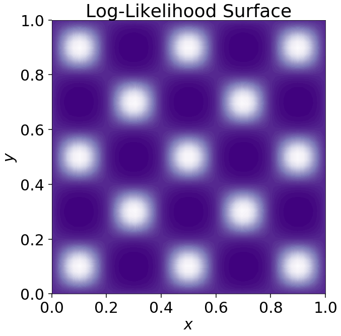
Consider a high-dimensional eggbox posterior, with two modes in each direction. Assuming 20 parameters, this give \(2^{20} \sim 10^6\) modes.
We can effectively marginalize over likelihoods with 1 Mio modes, using only 10 thousand samples.
Even for our simple toy model parameter inference is very difficult, and common solutions require to either neglect point source emission or diffuse emission uncertainties.
The reason is that standard MCMC based methods fail in light of the large number of parametres.
Neural network based solutions can instead “directly jump to the conclusion” and estimate marginal posteriors for any parameter of interest, without penalty for model complexity/realism.
This is a GAME CHANGER, and it is happening right now. Good time to be a PhD student!
Step 3. How to draw conclusions
(this one will be really short)
How are discoveries made?
(D1) Evidence against the null hypotehsis
The false positive rate should be so low that we almost certainly do not look at statistical noise.
The signal should reproduce with more data.
(D2) No alternative hypothesis
Exclude known unknowns
No instrumental artefact, astrophyiscal backgrounds, etc
A popular statistical technique in indirect searches is frequentist statistics, and \(p\)-values. It can be used to quantify the evidence against the null (background-only) hypothesis.
The probability \(p\) that \(TS\) is at least as large (extreme) as observed is called \(p\)-value.
Warning: Frequentist statements indicate that systematic uncertainties are either negligible, or neglected.
Bayesian evidence
In a Bayesian context, we would perform model comparison. Typically we would compare a “background-only” model, \(H_0\), with a background+signal model, \(H_1\), and calculate the Bayes factor. \[
B = \frac{p(\mathbf x| H_1)}{p(\mathbf x|H_0)}
\]
Interpretations can be based on Jeffrey’s scale
Warning: There is still relatively little experience in making discoveries using Bayesian statistics only. Maybe this will change in the future, or hybrid methods will become popular.


 Sign
Sign Sigmoid
 ReLU
ReLU