class: left, middle # Neural networks and likelihood-free inference.red.bold[*] .center.width-60[] .right[ Christoph Weniger, GRAPPA University of Amsterdam 10 March 2020 ] .left.footnote[.red.bold[*] Based on the beautiful slide decks of [Gilles Louppe](https://glouppe.github.io/teaching.html).] --- class: middle # Overview .bold[ - Neural Networks - Gradient Descent and Automatic differentiation - [Ex 1: Logistic regression](#ex1) - Deep Neural Networks - [Ex 1b: Simple multilayer perceptron](#ex1b) - [Ex 2: General function approximation](#ex2) - Convolutional Neural Networks - [Ex 3: Convnet parameter regression](#ex3) - Inside convolutional neural networks - Neural likelihood-free inference - [Ex 4: Posterior estimation with Convnets](#ex4) ] --- class: middle # Neural Networks --- # Perceptron The perceptron model (Rosenblatt, 1957) $$f(\mathbf{x}) = \begin{cases} 1 &\text{if } \sum_i w_i x_i + b \geq 0 \\\\ 0 &\text{otherwise} \end{cases}$$ was originally motivated by biology, with $w_i$ being synaptic weights and $x_i$ and $f$ firing rates. --- exclude: true # Threshold Logic Unit .grid[ .kol-1-2[ For boolean inputs, any Boolean function can be implemented: - $\text{or}(a,b) = 1\_{\\\{a+b - 0.5 \geq 0\\\}}$ - $\text{and}(a,b) = 1\_{\\\{a+b - 1.5 \geq 0\\\}}$ - $\text{not}(a) = 1\_{\\\{-a + 0.5 \geq 0\\\}}$ ] .kol-1-2[ .center.width-60[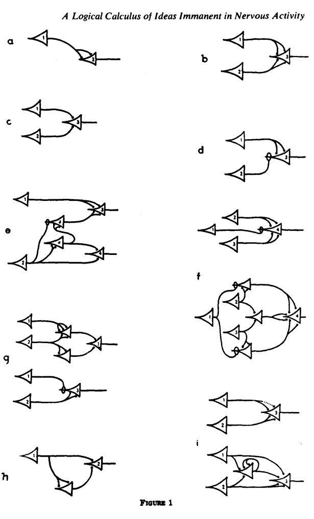] ] ] .footnote[Credits: McCulloch and Pitts, [A logical calculus of ideas immanent in nervous activity](http://www.cse.chalmers.se/~coquand/AUTOMATA/mcp.pdf), 1943.] --- class: middle .center.width-100[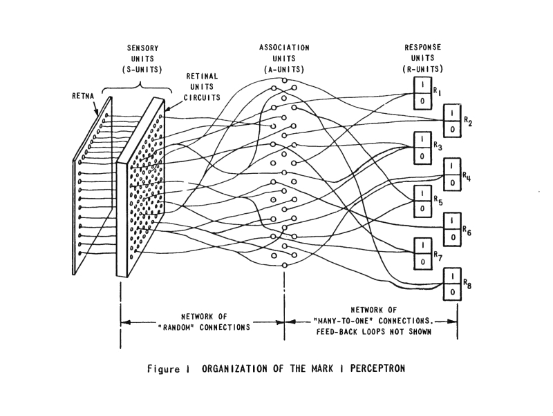] .footnote[Credits: Frank Rosenblatt, [Mark I Perceptron operators' manual](https://apps.dtic.mil/dtic/tr/fulltext/u2/236965.pdf), 1960.] ??? A perceptron is a signal transmission network consisting of sensory units (S units), association units (A units), and output or response units (R units). The ‘retina’ of the perceptron is an array of sensory elements (photocells). An S-unit produces a binary output depending on whether or not it is excited. A randomly selected set of retinal cells is connected to the next level of the network, the A units. As originally proposed there were extensive connections among the A units, the R units, and feedback between the R units and the A units. In essence an association unit is also an MCP neuron which is 1 if a single specific pattern of inputs is received, and it is 0 for all other possible patterns of inputs. Each association unit will have a certain number of inputs which are selected from all the inputs to the perceptron. So the number of inputs to a particular association unit does not have to be the same as the total number of inputs to the perceptron, but clearly the number of inputs to an association unit must be less than or equal to the total number of inputs to the perceptron. Each association unit's output then becomes the input to a single MCP neuron, and the output from this single MCP neuron is the output of the perceptron. So a perceptron consists of a "layer" of MCP neurons, and all of these neurons send their output to a single MCP neuron. --- class: middle, center, black-slide .grid[ .kol-1-2[.width-100[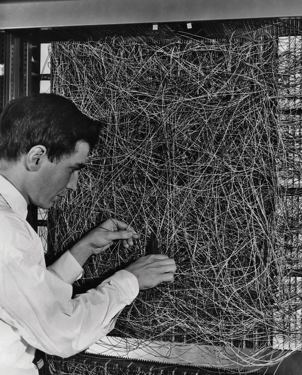]] .kol-1-2[<br><br>.width-100[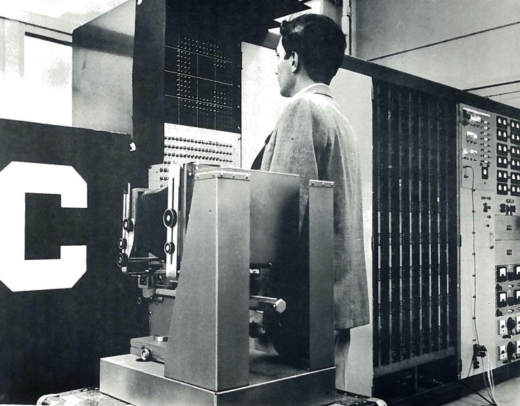]] ] The Mark I Percetron (Frank Rosenblatt). --- class: middle, center, black-slide <iframe width="600" height="450" src="https://www.youtube.com/embed/cNxadbrN_aI" frameborder="0" allowfullscreen></iframe> The Perceptron --- class: middle Let us define the (non-linear) **activation** function: $$\text{sign}(x) = \begin{cases} 1 &\text{if } x \geq 0 \\\\ 0 &\text{otherwise} \end{cases}$$ .center[] The perceptron classification rule can be rewritten as $$f(\mathbf{x}) = \text{sign}(\sum\_i w\_i x\_i + b).$$ --- class: middle ## Computational graphs .grid[ .kol-3-5[.width-90[]] .kol-2-5[ The computation of $$f(\mathbf{x}) = \text{sign}(\sum\_i w\_i x\_i + b)$$ can be represented as a **computational graph** where - white nodes correspond to inputs and outputs; - red nodes correspond to model parameters; - blue nodes correspond to intermediate operations. ] ] ??? Draw the NN diagram. --- class: middle In terms of **tensor operations**, $f$ can be rewritten as $$f(\mathbf{x}) = \text{sign}(\mathbf{w}^T \mathbf{x} + b),$$ for which the corresponding computational graph of $f$ is: .center.width-70[] --- exclude: true # Linear discriminant analysis Consider training data $(\mathbf{x}, y) \sim P(X,Y)$, with - $\mathbf{x} \in \mathbb{R}^p$, - $y \in \\\{0,1\\\}$. Assume class populations are Gaussian, with same covariance matrix $\Sigma$ (homoscedasticity): $$P(\mathbf{x}|y) = \frac{1}{\sqrt{(2\pi)^p |\Sigma|}} \exp \left(-\frac{1}{2}(\mathbf{x} - \mathbf{\mu}_y)^T \Sigma^{-1}(\mathbf{x} - \mathbf{\mu}_y) \right)$$ --- exclude: true <br> Using the Bayes' rule, we have: $$ \begin{aligned} P(Y=1|\mathbf{x}) &= \frac{P(\mathbf{x}|Y=1) P(Y=1)}{P(\mathbf{x})} \\\\ &= \frac{P(\mathbf{x}|Y=1) P(Y=1)}{P(\mathbf{x}|Y=0)P(Y=0) + P(\mathbf{x}|Y=1)P(Y=1)} \\\\ &= \frac{1}{1 + \frac{P(\mathbf{x}|Y=0)P(Y=0)}{P(\mathbf{x}|Y=1)P(Y=1)}}. \end{aligned} $$ -- exclude: true count: false It follows that with $$\sigma(x) = \frac{1}{1 + \exp(-x)},$$ we get $$P(Y=1|\mathbf{x}) = \sigma\left(\log \frac{P(\mathbf{x}|Y=1)}{P(\mathbf{x}|Y=0)} + \log \frac{P(Y=1)}{P(Y=0)}\right).$$ --- exclude: true class: middle Therefore, $$\begin{aligned} &P(Y=1|\mathbf{x}) \\\\ &= \sigma\left(\log \frac{P(\mathbf{x}|Y=1)}{P(\mathbf{x}|Y=0)} + \underbrace{\log \frac{P(Y=1)}{P(Y=0)}}\_{a}\right) \\\\ &= \sigma\left(\log P(\mathbf{x}|Y=1) - \log P(\mathbf{x}|Y=0) + a\right) \\\\ &= \sigma\left(-\frac{1}{2}(\mathbf{x} - \mathbf{\mu}\_1)^T \Sigma^{-1}(\mathbf{x} - \mathbf{\mu}\_1) + \frac{1}{2}(\mathbf{x} - \mathbf{\mu}\_0)^T \Sigma^{-1}(\mathbf{x} - \mathbf{\mu}\_0) + a\right) \\\\ &= \sigma\left(\underbrace{(\mu\_1-\mu\_0)^T \Sigma^{-1}}\_{\mathbf{w}^T}\mathbf{x} + \underbrace{\frac{1}{2}(\mu\_0^T \Sigma^{-1} \mu\_0 - \mu\_1^T \Sigma^{-1} \mu\_1) + a}\_{b} \right) \\\\ &= \sigma\left(\mathbf{w}^T \mathbf{x} + b\right) \end{aligned}$$ --- exclude: true class: middle, center .width-100[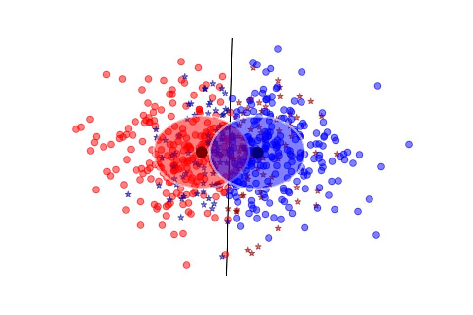] --- exclude: true count: false class: middle, center .width-100[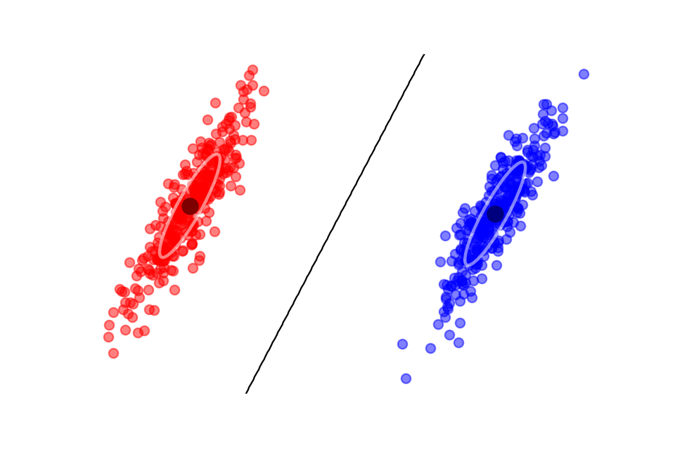] --- # The sigmoid function .footnote[This is also motivated by linear discriminat analysis.] .kol-1-2[ Extending binary logic with Bayesian probabilities motivates the **sigmoid** function, $$\sigma(x) = \frac{1}{1 + \exp(-x)}$$ which looks like a soft heavyside. Therefore, an overall model $f(\mathbf{x};\mathbf{w},b) = \sigma(\mathbf{w}^T \mathbf{x} + b)$ is very similar to the perceptron. ] .kol-1-2[ .center[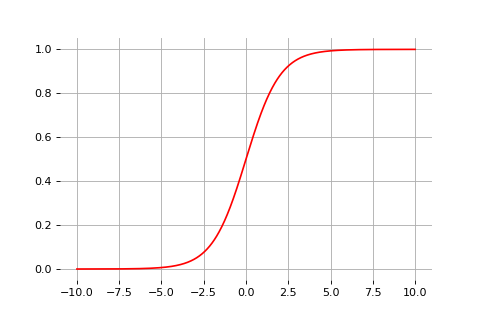] ] --- class: middle, center .center.width-70[] This unit is the main **primitive** of all neural networks! --- # Example: Logistic regression .grid[ .kol-1-2[ Consider the model $$P(Y=1|\mathbf{x}) = \sigma\left(\mathbf{w}^T \mathbf{x} + b\right)$$. - colored classes correspond to $Y=1$ and $Y=0$ - no model assumptions on class population (Gaussian class populations, homoscedasticity); - goal: instead, find $\mathbf{w}, b$ that maximizes the likelihood of the data. ] .kol-1-2[ .width-100[] ]] --- name: loss1 class: middle We have, $$ \begin{aligned} &\arg \max\_{\mathbf{w},b} P(\mathbf{d}|\mathbf{w},b) \\\\ &= \arg \max\_{\mathbf{w},b} \prod\_{\mathbf{x}\_i, y\_i \in \mathbf{d}} P(Y=y\_i|\mathbf{x}\_i, \mathbf{w},b) \\\\ &= \arg \max\_{\mathbf{w},b} \prod\_{\mathbf{x}\_i, y\_i \in \mathbf{d}} \sigma(\mathbf{w}^T \mathbf{x}\_i + b)^{y\_i} (1-\sigma(\mathbf{w}^T \mathbf{x}\_i + b))^{1-y\_i} \\\\ &= \arg \min\_{\mathbf{w},b} \underbrace{\sum\_{\mathbf{x}\_i, y\_i \in \mathbf{d}} -{y\_i} \log\sigma(\mathbf{w}^T \mathbf{x}\_i + b) - {(1-y\_i)} \log (1-\sigma(\mathbf{w}^T \mathbf{x}\_i + b))}\_{\mathcal{L}(\mathbf{w}, b) = \sum\_i \ell(y\_i, \hat{y}(\mathbf{x}\_i; \mathbf{w}, b))} \end{aligned} $$ ??? This loss is an instance of the **cross-entropy** $$H(p,q) = \mathbb{E}_p[-\log q]$$ for $p=Y|\mathbf{x}\_i$ and $q=\hat{Y}|\mathbf{x}\_i$. --- exclude: true class: middle When $Y$ takes values in $\\{-1,1\\}$, a similar derivation yields the **logistic loss** $$\mathcal{L}(\mathbf{w}, b) = -\sum_{\mathbf{x}\_i, y\_i \in \mathbf{d}} \log \sigma\left(y\_i (\mathbf{w}^T \mathbf{x}\_i + b))\right).$$ .center[] --- class: middle - In general, the cross-entropy and the logistic losses do not admit a minimizer that can be expressed analytically in closed form. - However, a minimizer can be found numerically, using a general minimization technique such as **gradient descent**. --- class: middle # Gradient descent --- # Gradient descent Let $\mathcal{L}(\theta)$ denote a loss function defined over model parameters $\theta$ (e.g., $\mathbf{w}$ and $b$). To minimize $\mathcal{L}(\theta)$, **gradient descent** uses local linear information to iteratively move towards a (local) minimum. For $\theta\_0 \in \mathbb{R}^d$, a first-order approximation around $\theta\_0$ can be defined as $$\hat{\mathcal{L}}(\epsilon; \theta\_0) = \mathcal{L}(\theta\_0) + \epsilon^T\nabla\_\theta \mathcal{L}(\theta\_0) + \frac{1}{2\gamma}||\epsilon||^2.$$ .center.width-60[] --- class: middle A minimizer of the approximation $\hat{\mathcal{L}}(\epsilon; \theta\_0)$ is given for $$\begin{aligned} \nabla\_\epsilon \hat{\mathcal{L}}(\epsilon; \theta\_0) &= 0 \\\\ &= \nabla\_\theta \mathcal{L}(\theta\_0) + \frac{1}{\gamma} \epsilon, \end{aligned}$$ which results in the best improvement for the step $\epsilon = -\gamma \nabla\_\theta \mathcal{L}(\theta\_0)$. Therefore, model parameters can be updated iteratively using the update rule $$\theta\_{t+1} = \theta\_t -\gamma \nabla\_\theta \mathcal{L}(\theta\_t),$$ where - $\theta_0$ are the initial parameters of the model; - $\gamma$ is the **learning rate**; - both are critical for the convergence of the update rule. --- class: center, middle  Example 1: Convergence to a local minima --- count: false class: center, middle  Example 1: Convergence to a local minima --- count: false class: center, middle  Example 1: Convergence to a local minima --- count: false class: center, middle  Example 1: Convergence to a local minima --- count: false class: center, middle  Example 1: Convergence to a local minima --- count: false class: center, middle  Example 1: Convergence to a local minima --- count: false class: center, middle  Example 1: Convergence to a local minima --- count: false class: center, middle  Example 1: Convergence to a local minima --- class: center, middle  Example 2: Convergence to the global minima --- count: false class: center, middle  Example 2: Convergence to the global minima --- count: false class: center, middle  Example 2: Convergence to the global minima --- count: false class: center, middle  Example 2: Convergence to the global minima --- count: false class: center, middle  Example 2: Convergence to the global minima --- count: false class: center, middle  Example 2: Convergence to the global minima --- count: false class: center, middle  Example 2: Convergence to the global minima --- count: false class: center, middle  Example 2: Convergence to the global minima --- class: center, middle  Example 3: Divergence due to a too large learning rate --- count: false class: center, middle  Example 3: Divergence due to a too large learning rate --- count: false class: center, middle  Example 3: Divergence due to a too large learning rate --- count: false class: center, middle  Example 3: Divergence due to a too large learning rate --- count: false class: center, middle  Example 3: Divergence due to a too large learning rate --- count: false class: center, middle  Example 3: Divergence due to a too large learning rate --- # Stochastic gradient descent In the empirical risk minimization setup, $\mathcal{L}(\theta)$ and its gradient decompose as $$\begin{aligned} \mathcal{L}(\theta) &= \frac{1}{N} \sum\_{\mathbf{x}\_i, y\_i \in \mathbf{d}} \ell(y\_i, f(\mathbf{x}\_i; \theta)) \\\\ \nabla \mathcal{L}(\theta) &= \frac{1}{N} \sum\_{\mathbf{x}\_i, y\_i \in \mathbf{d}} \nabla \ell(y\_i, f(\mathbf{x}\_i; \theta)). \end{aligned}$$ Therefore, in **batch** gradient descent the complexity of an update grows linearly with the size $N$ of the dataset. This is bad! --- class: middle Since the empirical risk is already an approximation of the expected risk, it should not be necessary to carry out the minimization with great accuracy. --- <br><br> Instead, **stochastic** gradient descent uses as update rule: $$\theta\_{t+1} = \theta\_t - \gamma \nabla \ell(y\_{i(t+1)}, f(\mathbf{x}\_{i(t+1)}; \theta\_t))$$ - Iteration complexity is independent of $N$. - The stochastic process $\\\{ \theta\_t | t=1, ... \\\}$ depends on the examples $i(t)$ picked randomly at each iteration. -- .grid.center.italic[ .kol-1-2[.width-100[] Batch gradient descent] .kol-1-2[.width-100[] Stochastic gradient descent ] ] --- exclude: true class: middle Why is stochastic gradient descent still a good idea? - Informally, averaging the update $$\theta\_{t+1} = \theta\_t - \gamma \nabla \ell(y\_{i(t+1)}, f(\mathbf{x}\_{i(t+1)}; \theta\_t)) $$ over all choices $i(t+1)$ restores batch gradient descent. - Formally, if the gradient estimate is **unbiased**, e.g., if $$\begin{aligned} \mathbb{E}\_{i(t+1)}[\nabla \ell(y\_{i(t+1)}, f(\mathbf{x}\_{i(t+1)}; \theta\_t))] &= \frac{1}{N} \sum\_{\mathbf{x}\_i, y\_i \in \mathbf{d}} \nabla \ell(y\_i, f(\mathbf{x}\_i; \theta\_t)) \\\\ &= \nabla \mathcal{L}(\theta\_t) \end{aligned}$$ then the formal convergence of SGD can be proved, under appropriate assumptions (see references). - If training is limited to single pass over the data, then SGD directly minimizes the **expected** risk. --- exclude: true class: middle The excess error characterizes the expected risk discrepancy between the Bayes model and the approximate empirical risk minimizer. It can be decomposed as $$\begin{aligned} &\mathbb{E}\left[ R(\tilde{f}\_\*^\mathbf{d}) - R(f\_B) \right] \\\\ &= \mathbb{E}\left[ R(f\_\*) - R(f\_B) \right] + \mathbb{E}\left[ R(f\_\*^\mathbf{d}) - R(f\_\*) \right] + \mathbb{E}\left[ R(\tilde{f}\_\*^\mathbf{d}) - R(f\_\*^\mathbf{d}) \right] \\\\ &= \mathcal{E}\_\text{app} + \mathcal{E}\_\text{est} + \mathcal{E}\_\text{opt} \end{aligned}$$ where - $\mathcal{E}\_\text{app}$ is the approximation error due to the choice of an hypothesis space, - $\mathcal{E}\_\text{est}$ is the estimation error due to the empirical risk minimization principle, - $\mathcal{E}\_\text{opt}$ is the optimization error due to the approximate optimization algorithm. --- exclude: true class: middle A fundamental result due to Bottou and Bousquet (2011) states that stochastic optimization algorithms (e.g., SGD) yield the best generalization performance (in terms of excess error) despite being the worst optimization algorithms for minimizing the empirical risk. --- # Automatic differentiation To minimize $\mathcal{L}(\theta)$ with stochastic gradient descent, we need the gradient $\nabla_\theta \mathcal{\ell}(\theta_t)$. Therefore, we require the evaluation of the (total) derivatives $$\frac{\text{d} \ell}{\text{d} \mathbf{W}\_k} \,\text{and}\, \frac{\text{d} \mathcal{\ell}}{\text{d} \mathbf{b}\_k}$$ of the loss $\ell$ with respect to all model parameters $\mathbf{W}\_k$, $\mathbf{b}\_k$, for $k=1, ..., L$. These derivatives can be evaluated automatically from the *computational graph* of $\ell$ using **automatic differentiation**. --- class: middle ## Chain rule .center.width-60[] Let us consider a 1-dimensional output composition $f \circ g$, such that $$\begin{aligned} y &= f(\mathbf{u}) \\\\ \mathbf{u} &= g(x) = (g\_1(x), ..., g\_m(x)). \end{aligned}$$ --- class: middle The **chain rule** states that $(f \circ g)' = (f' \circ g) g'.$ For the total derivative, the chain rule generalizes to $$ \begin{aligned} \frac{\text{d} y}{\text{d} x} &= \sum\_{k=1}^m \frac{\partial y}{\partial u\_k} \underbrace{\frac{\text{d} u\_k}{\text{d} x}}\_{\text{recursive case}} \end{aligned}$$ --- class: middle ## Reverse automatic differentiation - Since a neural network is a **composition of differentiable functions**, the total derivatives of the loss can be evaluated backward, by applying the chain rule recursively over its computational graph. - The implementation of this procedure is called reverse *automatic differentiation*. --- name: ex1 # .red[Exercise 1: Logistic regression] .center[[SOLUTION](https://colab.research.google.com/drive/1WjNYyYnhurEZWhUvposJfgASZBFvFnJ1)] Your task is to train a logistic regression model to predict the gender based on height and weight information only. The three-column training data can be downloaded [here](https://raw.githubusercontent.com/johnmyleswhite/ML_for_Hackers/master/02-Exploration/data/01_heights_weights_genders.csv). .grid[ .kol-1-2[ .center.width-80[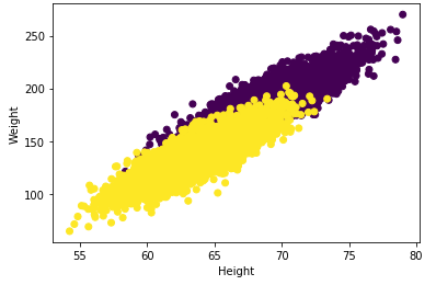] ] .kol-1-2[ ```csv "Gender","Height","Weight" "Male",73.847017017515,241.893563180437 "Male",68.7819040458903,162.310472521300 ... "Female",60.6748561538626,128.615808477141 "Female",65.3866908281118,154.239363331212 ... ``` ] ] The model should predict for abritrary $(H, W)$ input pairs the probability of Female gender. --- class: middle ## Some tips You can solve this exercise however you like, it will simplify your life later in this lecture if you use `pytorch`. Recommended to define logistic regression model as `torch` Module. ```python # Logistic model class Net(nn.Module): def __init__(self): super(Net, self).__init__() self.fc1 = nn.Linear(2, 1) def forward(self, x): return torch.sigmoid(self.fc1(x)) ``` - Minimize the loss function $\mathcal{l}$ that you can find [here](#loss1). - Starting template in Google colab can be found [here](https://colab.research.google.com/drive/1WN26BBI07_irmG243Ttl9bzVr7ssgv3u) - Use `torch.optim.SGD` for parameter optimization - Confirm that normalizing data (subtracting mean, dividing by standard deviation) accelerates learning Check out [DEEP LEARNING WITH PYTORCH: A 60 MINUTE BLITZ](https://pytorch.org/tutorials/beginner/deep_learning_60min_blitz.html) for details. .footnote[Based on Conway and Myles, Machine Learning for Hackers book, Chapter 2] --- class: middle # Deep neural networks --- # Multi-layer perceptron So far we considered the logistic unit $h=\sigma\left(\mathbf{w}^T \mathbf{x} + b\right)$, where $h \in \mathbb{R}$, $\mathbf{x} \in \mathbb{R}^p$, $\mathbf{w} \in \mathbb{R}^p$ and $b \in \mathbb{R}$. These units can be composed *in parallel* to form a **layer** with $q$ outputs: $$\mathbf{h} = \sigma(\mathbf{W}^T \mathbf{x} + \mathbf{b})$$ where $\mathbf{h} \in \mathbb{R}^q$, $\mathbf{x} \in \mathbb{R}^p$, $\mathbf{W} \in \mathbb{R}^{p\times q}$, $b \in \mathbb{R}^q$ and where $\sigma(\cdot)$ is upgraded to the element-wise sigmoid function. <br> .center.width-70[] ??? Draw the NN diagram. --- class: middle Similarly, layers can be composed *in series*, such that: $$\begin{aligned} \mathbf{h}\_0 &= \mathbf{x} \\\\ \mathbf{h}\_1 &= \sigma(\mathbf{W}\_1^T \mathbf{h}\_0 + \mathbf{b}\_1) \\\\ ... \\\\ \mathbf{h}\_L &= \sigma(\mathbf{W}\_L^T \mathbf{h}\_{L-1} + \mathbf{b}\_L) \\\\ f(\mathbf{x}; \theta) = \hat{y} &= \mathbf{h}\_L \end{aligned}$$ where $\theta$ denotes the model parameters $\\{ \mathbf{W}\_k, \mathbf{b}\_k, ... | k=1, ..., L\\}$. This model is the **multi-layer perceptron**, also known as the fully connected feedforward network. ??? Draw the NN diagram. --- class: middle, center .width-100[] --- class: middle .width-100[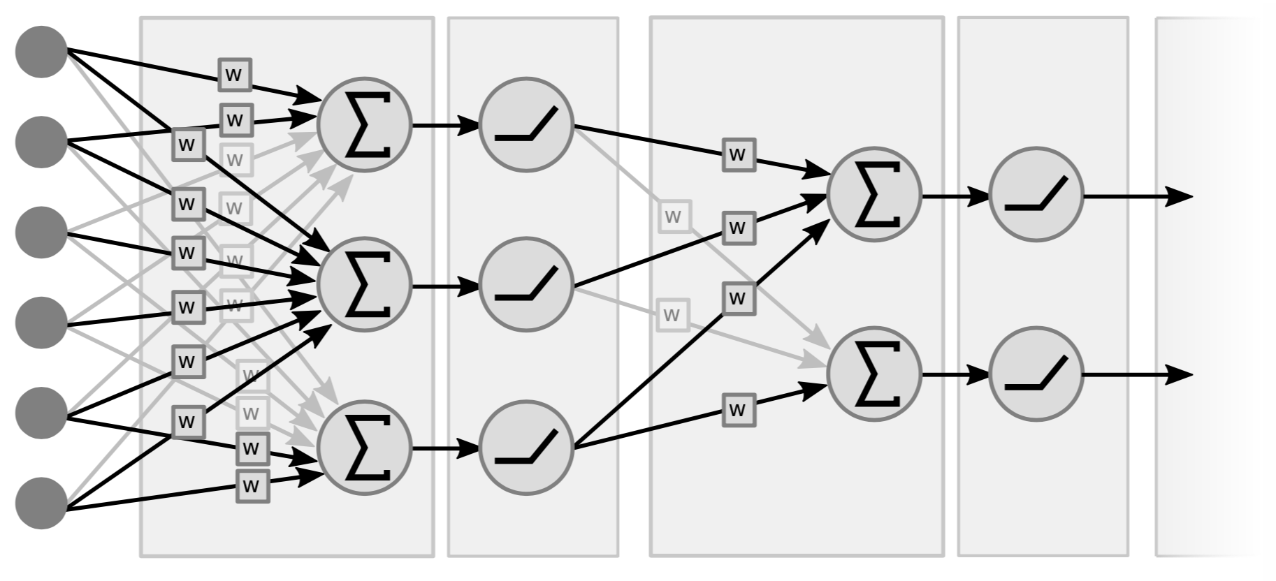] .footnote[Credits: [PyTorch Deep Learning Minicourse](https://atcold.github.io/pytorch-Deep-Learning-Minicourse/), Alfredo Canziani, 2020.] --- # Classification - For .red[binary classification], the width $q$ of the last layer $L$ is set to $1$, which results in a single output $h\_L \in [0,1]$ that models the probability $P(Y=1|\mathbf{x})$. - For .red[multi-class classification], the sigmoid action $\sigma$ in the last layer can be generalized to produce a vector $\mathbf{h}\_L \in \bigtriangleup^C$ of probability estimates $P(Y=i|\mathbf{x})$. <br><br> This activation is the $\text{Softmax}$ function, where its $i$-th output is defined as $$\text{Softmax}(\mathbf{z})\_i = \frac{\exp(z\_i)}{\sum\_{j=1}^C \exp(z\_j)},$$ for $i=1, ..., C$. --- # Regression For .red[regression problems], one usually starts with the assumption that $$P(y|\mathbf{x}) = \mathcal{N}(y; \mu=f(\mathbf{x}; \theta), \sigma^2=1),$$ where $f$ is parameterized with a neural network which last layer does not contain any final activation. --- class: middle We have, $$\begin{aligned} &\arg \max\_{\theta} P(\mathbf{d}|\theta) \\\\ &= \arg \max\_{\theta} \prod\_{\mathbf{x}\_i, y\_i \in \mathbf{d}} P(Y=y\_i|\mathbf{x}\_i, \theta) \\\\ &= \arg \min\_{\theta} -\sum\_{\mathbf{x}\_i, y\_i \in \mathbf{d}} \log P(Y=y\_i|\mathbf{x}\_i, \theta) \\\\ &= \arg \min\_{\theta} -\sum\_{\mathbf{x}\_i, y\_i \in \mathbf{d}} \log\left( \frac{1}{\sqrt{2\pi}} \exp\(-\frac{1}{2}(y\_i - f(\mathbf{x};\theta))^2\) \right)\\\\ &= \arg \min\_{\theta} \sum\_{\mathbf{x}\_i, y\_i \in \mathbf{d}} (y\_i - f(\mathbf{x};\theta))^2, \end{aligned}$$ which recovers the common **squared error** loss $\ell(y, \hat{y}) = (y-\hat{y})^2$. --- exclude: true class: middle Let us consider a simplified 2-layer MLP and the following loss function: $$\begin{aligned} f(\mathbf{x}; \mathbf{W}\_1, \mathbf{W}\_2) &= \sigma\left( \mathbf{W}\_2^T \sigma\left( \mathbf{W}\_1^T \mathbf{x} \right)\right) \\\\ \mathcal{\ell}(y, \hat{y}; \mathbf{W}\_1, \mathbf{W}\_2) &= \text{cross\\\_ent}(y, \hat{y}) + \lambda \left( ||\mathbf{W}_1||\_2 + ||\mathbf{W}\_2||\_2 \right) \end{aligned}$$ for $\mathbf{x} \in \mathbb{R^p}$, $y \in \mathbb{R}$, $\mathbf{W}\_1 \in \mathbb{R}^{p \times q}$ and $\mathbf{W}\_2 \in \mathbb{R}^q$. --- exclude: true class: middle In the *forward pass*, intermediate values are all computed from inputs to outputs, which results in the annotated computational graph below: .width-100[] --- exclude: true class: middle The total derivative can be computed through a **backward pass**, by walking through all paths from outputs to parameters in the computational graph and accumulating the terms. For example, for $\frac{\text{d} \ell}{\text{d} \mathbf{W}\_1}$ we have: $$\begin{aligned} \frac{\text{d} \ell}{\text{d} \mathbf{W}\_1} &= \frac{\partial \ell}{\partial u\_8}\frac{\text{d} u\_8}{\text{d} \mathbf{W}\_1} + \frac{\partial \ell}{\partial u\_4}\frac{\text{d} u\_4}{\text{d} \mathbf{W}\_1} \\\\ \frac{\text{d} u\_8}{\text{d} \mathbf{W}\_1} &= ... \end{aligned}$$ .width-100[] --- exclude: true class: middle .width-100[] Let us zoom in on the computation of the network output $\hat{y}$ and of its derivative with respect to $\mathbf{W}\_1$. - *Forward pass*: values $u\_1$, $u\_2$, $u\_3$ and $\hat{y}$ are computed by traversing the graph from inputs to outputs given $\mathbf{x}$, $\mathbf{W}\_1$ and $\mathbf{W}\_2$. - **Backward pass**: by the chain rule we have $$\begin{aligned} \frac{\text{d} \hat{y}}{\text{d} \mathbf{W}\_1} &= \frac{\partial \hat{y}}{\partial u\_3} \frac{\partial u\_3}{\partial u\_2} \frac{\partial u\_2}{\partial u\_1} \frac{\partial u\_1}{\partial \mathbf{W}\_1} \\\\ &= \frac{\partial \sigma(u\_3)}{\partial u\_3} \frac{\partial \mathbf{W}\_2^T u\_2}{\partial u\_2} \frac{\partial \sigma(u\_1)}{\partial u\_1} \frac{\partial \mathbf{W}\_1^T \mathbf{x}}{\partial \mathbf{W}\_1} \end{aligned}$$ Note how evaluating the partial derivatives requires the intermediate values computed forward. --- exclude: true class: middle - This algorithm is also known as **backpropagation**. - An equivalent procedure can be defined to evaluate the derivatives in *forward mode*, from inputs to outputs. - Since differentiation is a linear operator, automatic differentiation can be implemented efficiently in terms of tensor operations. --- # The vanishing gradients problem Training deep MLPs with many layers has for long (pre-2011) been very difficult due to the **vanishing gradient** problem. - Small gradients slow down, and eventually block, stochastic gradient descent. - This results in a limited capacity of learning. .width-100[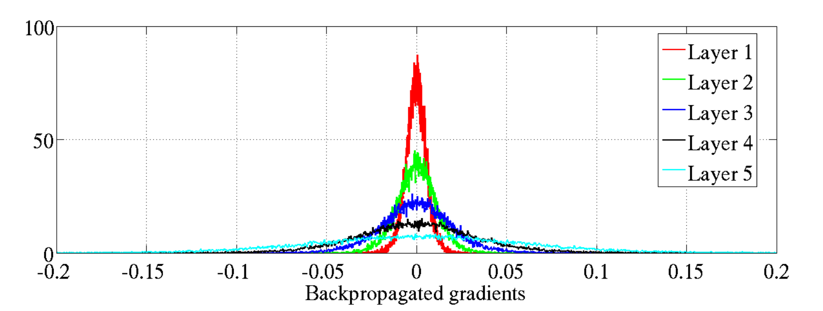] .caption[Backpropagated gradients normalized histograms (Glorot and Bengio, 2010).<br> Gradients for layers far from the output vanish to zero. ] --- exclude: true class: middle Let us consider a simplified 3-layer MLP, with $x, w\_1, w\_2, w\_3 \in\mathbb{R}$, such that $$f(x; w\_1, w\_2, w\_3) = \sigma\left(w\_3\sigma\left( w\_2 \sigma\left( w\_1 x \right)\right)\right). $$ Under the hood, this would be evaluated as $$\begin{aligned} u\_1 &= w\_1 x \\\\ u\_2 &= \sigma(u\_1) \\\\ u\_3 &= w\_2 u\_2 \\\\ u\_4 &= \sigma(u\_3) \\\\ u\_5 &= w\_3 u\_4 \\\\ \hat{y} &= \sigma(u\_5) \end{aligned}$$ and its derivative $\frac{\text{d}\hat{y}}{\text{d}w\_1}$ as $$\begin{aligned}\frac{\text{d}\hat{y}}{\text{d}w\_1} &= \frac{\partial \hat{y}}{\partial u\_5} \frac{\partial u\_5}{\partial u\_4} \frac{\partial u\_4}{\partial u\_3} \frac{\partial u\_3}{\partial u\_2}\frac{\partial u\_2}{\partial u\_1}\frac{\partial u\_1}{\partial w\_1}\\\\ &= \frac{\partial \sigma(u\_5)}{\partial u\_5} w\_3 \frac{\partial \sigma(u\_3)}{\partial u\_3} w\_2 \frac{\partial \sigma(u\_1)}{\partial u\_1} x \end{aligned}$$ --- class: middle The derivative of the sigmoid activation function $\sigma$ is: .center[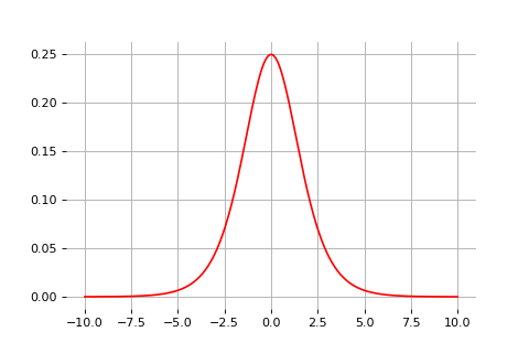] $$\frac{\text{d} \sigma}{\text{d} x}(x) = \sigma(x)(1-\sigma(x))$$ Notice that $0 \leq \frac{\text{d} \sigma}{\text{d} x}(x) \leq \frac{1}{4}$ for all $x$. --- exclude: true class: middle Assume that weights $w\_1, w\_2, w\_3$ are initialized randomly from a Gaussian with zero-mean and small variance, such that with high probability $-1 \leq w\_i \leq 1$. Then, $$\frac{\text{d}\hat{y}}{\text{d}w\_1} = \underbrace{\frac{\partial \sigma(u\_5)}{\partial u\_5}}\_{\leq \frac{1}{4}} \underbrace{w\_3}\_{\leq 1} \underbrace{\frac{\partial \sigma(u\_3)}{\partial u\_3}}\_{\leq \frac{1}{4}} \underbrace{w\_2}\_{\leq 1} \underbrace{\frac{\sigma(u\_1)}{\partial u\_1}}\_{\leq \frac{1}{4}} x$$ This implies that the gradient $\frac{\text{d}\hat{y}}{\text{d}w\_1}$ **exponentially** shrinks to zero as the number of layers in the network increases. Hence the vanishing gradient problem. - In general, bounded activation functions (sigmoid, tanh, etc) are prone to the vanishing gradient problem. - Note the importance of a proper initialization scheme. --- # Rectified linear units Instead of the sigmoid activation function, modern neural networks are for most based on **rectified linear units** (ReLU) (Glorot et al, 2011): $$\text{ReLU}(x) = \max(0, x)$$ .center[] --- class: middle Note that the derivative of the ReLU function is $$\frac{\text{d}}{\text{d}x} \text{ReLU}(x) = \begin{cases} 0 &\text{if } x \leq 0 \\\\ 1 &\text{otherwise} \end{cases}$$ .center[] For $x=0$, the derivative is undefined. In practice, it is set to zero. --- exclude: true class: middle Therefore, $$\frac{\text{d}\hat{y}}{\text{d}w\_1} = \underbrace{\frac{\partial \sigma(u\_5)}{\partial u\_5}}\_{= 1} w\_3 \underbrace{\frac{\partial \sigma(u\_3)}{\partial u\_3}}\_{= 1} w\_2 \underbrace{\frac{\partial \sigma(u\_1)}{\partial u\_1}}\_{= 1} x$$ This **solves** the vanishing gradient problem, even for deep networks! (provided proper initialization) Note that: - The ReLU unit dies when its input is negative, which might block gradient descent. - This is actually a useful property to induce *sparsity*. - This issue can also be solved using **leaky** ReLUs, defined as $$\text{LeakyReLU}(x) = \max(\alpha x, x)$$ for a small $\alpha \in \mathbb{R}^+$ (e.g., $\alpha=0.1$). --- # Universal approximation (teaser) Let us consider the 1-layer MLP $$f(x) = \sum w\_i \text{ReLU}(x + b_i).$$ This model can approximate *any* smooth 1D function, provided enough hidden units. --- class: middle .center[] --- class: middle count: false .center[] --- class: middle count: false .center[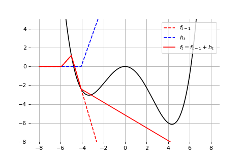] --- class: middle count: false .center[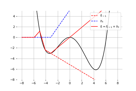] --- class: middle count: false .center[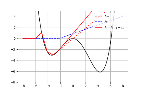] --- class: middle count: false .center[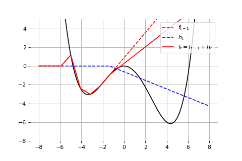] --- class: middle count: false .center[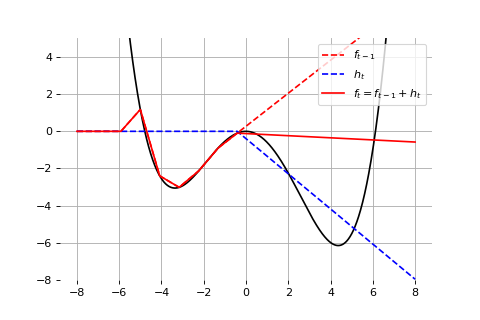] --- class: middle count: false .center[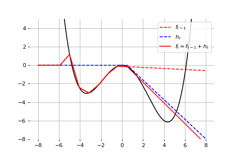] --- class: middle count: false .center[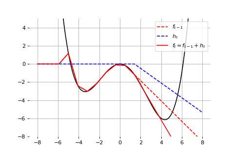] --- class: middle count: false .center[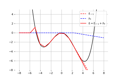] --- class: middle count: false .center[] --- class: middle count: false .center[] --- class: middle count: false .center[] --- name: ex1b # .red[Exercise 1b: Simple multilayer perceptron] Your task is to improve our logistic regression model by replacing the single affine transformation with a simple hidden layer model. Start with the solution to [exercise 1](#ex1). Replace .center[ $\texttt{INPUT} \to \texttt{FC} \to \texttt{SIGMOID} \to \texttt{OUTPUT}$ $\Rightarrow$ $\texttt{INPUT} \to \texttt{FC} \to \texttt{RELU} \to \texttt{FC} \to \texttt{SIGMOID} \to \texttt{OUTPUT}$ ] --- name: ex2 # .red[Exercise 2: Function approximators] Your task is to write a 2-layer dense neural network that approximates simple analytic functions on a grid $x_i$, $$ f_i(a, b) \equiv f(x_i,a, b) $$ for instance $$ f(x, a, b) = a\sin(x+b) $$ over the domain $x \in [-5, 5]$, and $a, b \in [0, 1]$. ## Tasks - Start with a copy of the [logistic regression example](#ex1b) - Use a neural network with one hidden layer, $\texttt{INPUT} \to \texttt{FC} \to \texttt{RELU} \to \texttt{FC} \to \texttt{OUTPUT}$. - Plot the function predict by your neural network in direct comparison with the training function. - Investigate the quality of the result for different hidden layer dimensions. --- class: middle, center ## Example (poorly trained)  --- class: middle # Convolutional neural networks --- class: middle # A little history --- class: middle ## Visual perception (Hubel and Wiesel, 1959-1962) - David Hubel and Torsten Wiesel discover the neural basis of **visual perception**. - Awarded the Nobel Prize of Medicine in 1981 for their discovery. .grid.center[ .kol-4-5.center[.width-80[]] .kol-1-5[<br>.width-100.circle[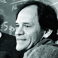].width-100.circle[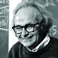]] ] --- class: middle, black-slide .center[ <iframe width="640" height="480" src="https://www.youtube.com/embed/IOHayh06LJ4?&loop=1&start=0" frameborder="0" volume="0" allowfullscreen></iframe> ] .center[Hubel and Wiesel] --- class: middle, black-slide .center[ <iframe width="640" height="480" src="https://www.youtube.com/embed/y_l4kQ5wjiw?&loop=1&start=97" frameborder="0" volume="0" allowfullscreen></iframe> ] .center[Hubel and Wiesel] ??? During their recordings, they noticed a few interesting things: 1. the neurons fired only when the line was in a particular place on the retina, 2. the activity of these neurons changed depending on the orientation of the line, and 3. sometimes the neurons fired only when the line was moving in a particular direction. --- class: middle .width-100.center[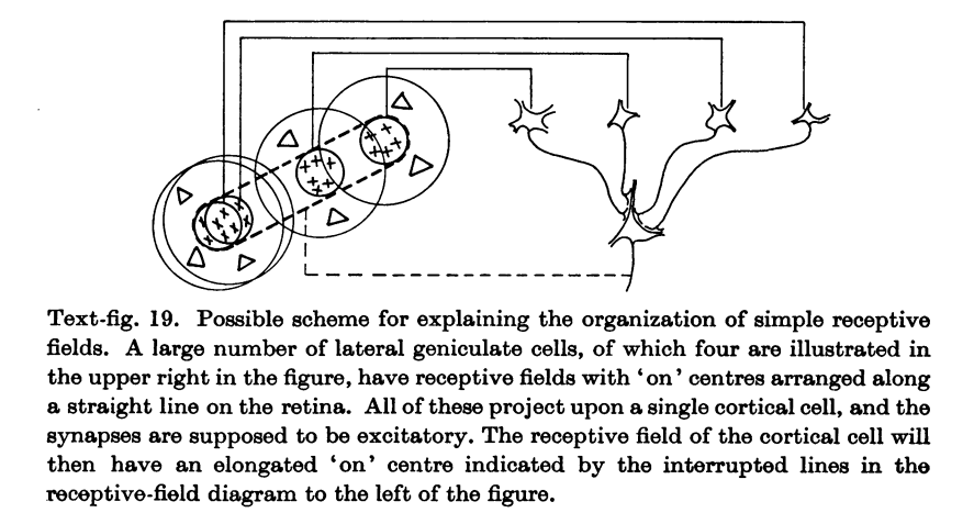] .footnote[Credits: Hubel and Wiesel, [Receptive fields, binocular interaction and functional architecture in the cat's visual cortex](https://www.ncbi.nlm.nih.gov/pmc/articles/PMC1359523/), 1962.] --- class: middle .width-100.center[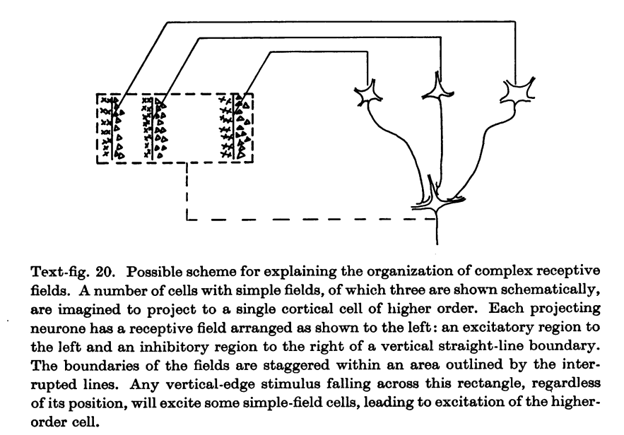] .footnote[Credits: Hubel and Wiesel, [Receptive fields, binocular interaction and functional architecture in the cat's visual cortex](https://www.ncbi.nlm.nih.gov/pmc/articles/PMC1359523/), 1962.] --- class: middle ## The Mark-1 Perceptron (Rosenblatt, 1957-61) .center.width-80[] - Rosenblatt builds the first implementation of a neural network. - The network is an anlogic circuit. Parameters are potentiometers. .footnote[Credits: Frank Rosenblatt, [Principle of Neurodynamics](http://www.dtic.mil/dtic/tr/fulltext/u2/256582.pdf), 1961.] ??? --- class: middle .center.width-60[] .italic["If we show the perceptron a stimulus, say a square, and associate a response to that square, this response will immediately **generalize perfectly to all transforms** of the square under the transformation group [...]."] .footnote[Credits: Frank Rosenblatt, [Principle of Neurodynamics](http://www.dtic.mil/dtic/tr/fulltext/u2/256582.pdf), 1961.] ??? This is quite similar to Hubel and Wiesel's simple and complex cells! --- class: middle ## AI winter (Minsky and Papert, 1969+) - Minsky and Papert prove a series of impossibility results for the perceptron (or rather, a narrowly defined variant thereof). - **AI winter** follows. .center[.width-80[] .width-20[]] .footnote[Credits: Minsky and Papert, Perceptrons: an Introduction to Computational Geometry, 1969.] --- class: middle ## Automatic differentiation (Werbos, 1974) - Werbos formulate an arbitrary function as a computational graph. - Symbolic derivatives are computed by dynamic programming. .grid[ .kol-2-5[ .center.width-100[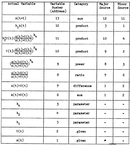] ] .kol-3-5[ <br> <br> .center.width-100[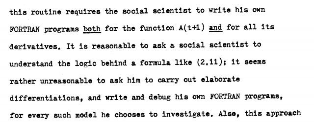] ] ] .footnote[Credits: [Paul Werbos, Beyond regression: new tools for prediction and analysis in the behavioral sciences, 1974.](https://www.researchgate.net/publication/35657389_Beyond_regression_new_tools_for_prediction_and_analysis_in_the_behavioral_sciences/link/576ac78508aef2a864d20964/download)] --- class: middle ## Neocognitron (Fukushima, 1980) .center.width-90[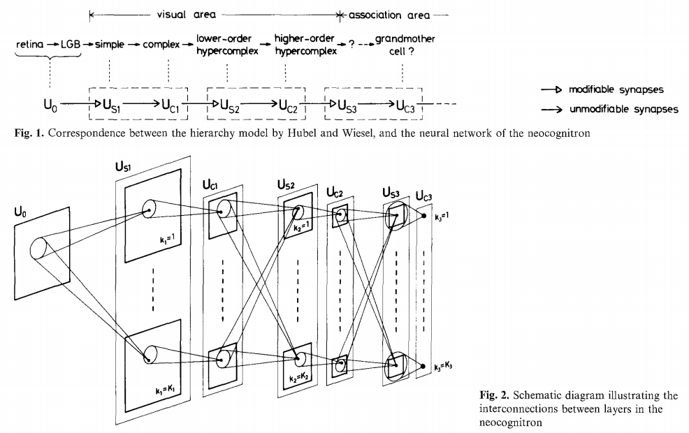] Fukushima proposes a direct neural network implementation of the hierarchy model of the visual nervous system of Hubel and Wiesel. .footnote[Credits: Kunihiko Fukushima, [Neocognitron: A Self-organizing Neural Network Model](https://www.rctn.org/bruno/public/papers/Fukushima1980.pdf), 1980.] --- class: middle .grid[ .kol-1-3.center[.width-100[] Convolutions] .kol-2-3.center[.width-100[] Feature hierarchy] ] .footnote[Credits: Kunihiko Fukushima, [Neocognitron: A Self-organizing Neural Network Model](https://www.rctn.org/bruno/public/papers/Fukushima1980.pdf), 1980.] ??? - Built upon **convolutions** and enables the composition of a *feature hierarchy*. - Biologically-inspired training algorithm, which proves to be largely **inefficient**. --- class: middle ## Backpropagation (Rumelhart et al, 1986) .grid[ .kol-1-2[ - Rumelhart and Hinton introduce **backpropagation** in multi-layer networks with sigmoid non-linearities and sum of squares loss function. - They advocate for batch gradient descent in supervised learning. - Discuss online gradient descent, momentum and random initialization. - Depart from *biologically plausible* training algorithms. ] .kol-1-2[ .center.width-100[] ] ] .footnote[Credits: Rumelhart et al, [Learning representations by back-propagating errors](http://www.cs.toronto.edu/~hinton/absps/naturebp.pdf), 1986.] --- class: middle ## Convolutional networks (LeCun, 1990) - LeCun trains a convolutional network by backpropagation. - He advocates for end-to-end feature learning in image classification. .center.width-70[] .footnote[Credits: LeCun et al, [Handwritten Digit Recognition with a Back-Propagation Network](http://yann.lecun.com/exdb/publis/pdf/lecun-90c.pdf), 1990.] --- class: middle, black-slide .center[ <iframe width="640" height="480" src="https://www.youtube.com/embed/FwFduRA_L6Q?&loop=1&start=0" frameborder="0" volume="0" allowfullscreen></iframe> ] .center[LeNet-1 (LeCun et al, 1993)] --- class: middle ## AlexNet (Krizhevsky et al, 2012) - Krizhevsky trains a convolutional network on ImageNet with two GPUs. - 16.4% top-5 error on ILSVRC'12, outperforming all other entries by 10% or more. - This event triggers the deep learning revolution. .center.width-100[] --- class: middle # Convolutions --- class: middle If they were handled as normal "unstructured" vectors, high-dimensional signals such as sound samples or images would require models of intractable size. E.g., a linear layer taking $256\times 256$ RGB images as input and producing an image of same size would require $$(256 \times 256 \times 3)^2 \approx 3.87e+10$$ parameters, with the corresponding memory footprint (150Gb!), and excess of capacity. .footnote[Credits: Francois Fleuret, [EE559 Deep Learning](https://fleuret.org/ee559/), EPFL.] --- class: middle This requirement is also inconsistent with the intuition that such large signals have some "invariance in translation". .bold[A representation meaningful at a certain location can / should be used everywhere]. A convolution layer embodies this idea. It applies the same linear transformation locally everywhere while preserving the signal structure. .footnote[Credits: Francois Fleuret, [EE559 Deep Learning](https://fleuret.org/ee559/), EPFL.] --- class: middle .center[] .footnote[Credits: Francois Fleuret, [EE559 Deep Learning](https://fleuret.org/ee559/), EPFL.] --- # Convolutions For one-dimensional tensors, given an input vector $\mathbf{x} \in \mathbb{R}^W$ and a convolutional kernel $\mathbf{u} \in \mathbb{R}^w$, the discrete **convolution** $\mathbf{x} \circledast \mathbf{u}$ is a vector of size $W - w + 1$ such that $$\begin{aligned} (\mathbf{x} \circledast \mathbf{u})[i] &= \sum\_{m=0}^{w-1} x\_{m+i} u\_m . \end{aligned} $$ ## Note Technically, $\circledast$ denotes the cross-correlation operator. However, most machine learning libraries call it convolution. --- class: middle Convolutions can implement differential operators: $$(0,0,0,0,1,2,3,4,4,4,4) \circledast (-1,1) = (0,0,0,1,1,1,1,0,0,0) $$ .center.width-100[] or crude template matchers: .center.width-100[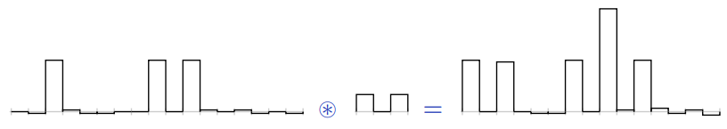] .footnote[Credits: Francois Fleuret, [EE559 Deep Learning](https://fleuret.org/ee559/), EPFL.] --- class: middle Convolutions generalize to multi-dimensional tensors: - In its most usual form, a convolution takes as input a 3D tensor $\mathbf{x} \in \mathbb{R}^{C \times H \times W}$, called the **input feature map**. - A kernel $\mathbf{u} \in \mathbb{R}^{C \times h \times w}$ slides across the input feature map, along its height and width. The size $h \times w$ is the size of the *receptive field*. - At each location, the element-wise product between the kernel and the input elements it overlaps is computed and the results are summed up. --- class: middle .center[] .footnote[Credits: Francois Fleuret, [EE559 Deep Learning](https://fleuret.org/ee559/), EPFL.] --- class: middle - The final output $\mathbf{o}$ is a 2D tensor of size $(H-h+1) \times (W-w+1)$ called the **output feature map** and such that: $$\begin{aligned} \mathbf{o}\_{j,i} &= \mathbf{b}\_{j,i} + \sum\_{c=0}^{C-1} (\mathbf{x}\_c \circledast \mathbf{u}\_c)[j,i] = \mathbf{b}\_{j,i} + \sum\_{c=0}^{C-1} \sum\_{n=0}^{h-1} \sum\_{m=0}^{w-1} \mathbf{x}\_{c,n+j,m+i} \mathbf{u}\_{c,n,m} \end{aligned}$$ where $\mathbf{u}$ and $\mathbf{b}$ are shared parameters to learn. - $D$ convolutions can be applied in the same way to produce a $D \times (H-h+1) \times (W-w+1)$ feature map, where $D$ is the depth. - Swiping across channels with a 3D convolution usually makes no sense, unless the channel index has some metric mearning. --- exclude: true class: middle Convolutions have three additional parameters: - The *padding* specifies the size of a zeroed frame added arount the input. - The **stride** specifies a step size when moving the kernel across the signal. - The *dilation* modulates the expansion of the filter without adding weights. .footnote[Credits: Francois Fleuret, [EE559 Deep Learning](https://fleuret.org/ee559/), EPFL.] --- exclude: true class: middle ## Padding Padding is useful to control the spatial dimension of the feature map, for example to keep it constant across layers. .center[ .width-45[] .width-45[] ] .footnote[Credits: Dumoulin and Visin, [A guide to convolution arithmetic for deep learning](https://arxiv.org/abs/1603.07285), 2016.] --- exclude: true class: middle ## Strides Stride is useful to reduce the spatial dimension of the feature map by a constant factor. .center[ .width-45[] ] .footnote[Credits: Dumoulin and Visin, [A guide to convolution arithmetic for deep learning](https://arxiv.org/abs/1603.07285), 2016.] --- exclude: true class: middle ## Dilation The dilation modulates the expansion of the kernel support by adding rows and columns of zeros between coefficients. Having a dilation coefficient greater than one increases the units receptive field size without increasing the number of parameters. .center[ .width-45[] ] .footnote[Credits: Dumoulin and Visin, [A guide to convolution arithmetic for deep learning](https://arxiv.org/abs/1603.07285), 2016.] --- # Equivariance A function $f$ is **equivariant** to $g$ if $f(g(\mathbf{x})) = g(f(\mathbf{x}))$. - Parameter sharing used in a convolutional layer causes the layer to be equivariant to translation. - That is, if $g$ is any function that translates the input, the convolution function is equivariant to $g$. .center.width-50[] .caption[If an object moves in the input image, its representation will move the same amount in the output.] .footnote[Credits: LeCun et al, Gradient-based learning applied to document recognition, 1998.] --- exclude: true class: middle - Equivariance is useful when we know some local function is useful everywhere (e.g., edge detectors). - Convolution is not equivariant to other operations such as change in scale or rotation. --- exclude: true # Convolutions as matrix multiplications As a guiding example, let us consider the convolution of single-channel tensors $\mathbf{x} \in \mathbb{R}^{4 \times 4}$ and $\mathbf{u} \in \mathbb{R}^{3 \times 3}$: $$ \mathbf{x} \circledast \mathbf{u} = \begin{pmatrix} 4 & 5 & 8 & 7 \\\\ 1 & 8 & 8 & 8 \\\\ 3 & 6 & 6 & 4 \\\\ 6 & 5 & 7 & 8 \end{pmatrix} \circledast \begin{pmatrix} 1 & 4 & 1 \\\\ 1 & 4 & 3 \\\\ 3 & 3 & 1 \end{pmatrix} = \begin{pmatrix} 122 & 148 \\\\ 126 & 134 \end{pmatrix}$$ --- exclude: true class: middle The convolution operation can be equivalently re-expressed as a single matrix multiplication: - the convolutional kernel $\mathbf{u}$ is rearranged as a **sparse Toeplitz circulant matrix**, called the convolution matrix: $$\mathbf{U} = \begin{pmatrix} 1 & 4 & 1 & 0 & 1 & 4 & 3 & 0 & 3 & 3 & 1 & 0 & 0 & 0 & 0 & 0 \\\\ 0 & 1 & 4 & 1 & 0 & 1 & 4 & 3 & 0 & 3 & 3 & 1 & 0 & 0 & 0 & 0 \\\\ 0 & 0 & 0 & 0 & 1 & 4 & 1 & 0 & 1 & 4 & 3 & 0 & 3 & 3 & 1 & 0 \\\\ 0 & 0 & 0 & 0 & 0 & 1 & 4 & 1 & 0 & 1 & 4 & 3 & 0 & 3 & 3 & 1 \end{pmatrix}$$ - the input $\mathbf{x}$ is flattened row by row, from top to bottom: $$v(\mathbf{x}) = \begin{pmatrix} 4 & 5 & 8 & 7 & 1 & 8 & 8 & 8 & 3 & 6 & 6 & 4 & 6 & 5 & 7 & 8 \end{pmatrix}^T$$ Then, $$\mathbf{U}v(\mathbf{x}) = \begin{pmatrix} 122 & 148 & 126 & 134 \end{pmatrix}^T$$ which we can reshape to a $2 \times 2$ matrix to obtain $\mathbf{x} \circledast \mathbf{u}$. --- exclude: true class: middle The same procedure generalizes to $\mathbf{x} \in \mathbb{R}^{H \times W}$ and convolutional kernel $\mathbf{u} \in \mathbb{R}^{h \times w}$, such that: - the convolutional kernel is rearranged as a sparse Toeplitz circulant matrix $\mathbf{U}$ of shape $(H-h+1)(W-w+1) \times HW$ where - each row $i$ identifies an element of the output feature map, - each column $j$ identifies an element of the input feature map, - the value $\mathbf{U}\_{i,j}$ corresponds to the kernel value the element $j$ is multiplied with in output $i$; - the input $\mathbf{x}$ is flattened into a column vector $v(\mathbf{x})$ of shape $HW \times 1$; - the output feature map $\mathbf{x} \circledast \mathbf{u}$ is obtained by reshaping the $(H-h+1)(W-w+1) \times 1$ column vector $\mathbf{U}v(\mathbf{x})$ as a $(H-h+1) \times (W-w+1)$ matrix. Therefore, a convolutional layer is a special case of a fully connected layer: $$\mathbf{h} = \mathbf{x} \circledast \mathbf{u} \Leftrightarrow v(\mathbf{h}) = \mathbf{U}v(\mathbf{x}) \Leftrightarrow v(\mathbf{h}) = \mathbf{W}^T v(\mathbf{x})$$ --- exclude: true class: middle, center  $$\Leftrightarrow$$  --- class: middle # Pooling --- class: middle When the input volume is large, **pooling layers** can be used to reduce the input dimension while preserving its global structure, in a way similar to a down-scaling operation. --- # Pooling Consider a pooling area of size $h \times w$ and a 3D input tensor $\mathbf{x} \in \mathbb{R}^{C\times(rh)\times(sw)}$. - Max-pooling produces a tensor $\mathbf{o} \in \mathbb{R}^{C \times r \times s}$ such that $$\mathbf{o}\_{c,j,i} = \max\_{n < h, m < w} \mathbf{x}_{c,rj+n,si+m}.$$ - Average pooling produces a tensor $\mathbf{o} \in \mathbb{R}^{C \times r \times s}$ such that $$\mathbf{o}\_{c,j,i} = \frac{1}{hw} \sum\_{n=0}^{h-1} \sum\_{m=0}^{w-1} \mathbf{x}_{c,rj+n,si+m}.$$ Pooling is very similar in its formulation to convolution. --- class: middle .center[] .footnote[Credits: Francois Fleuret, [EE559 Deep Learning](https://fleuret.org/ee559/), EPFL.] --- # Invariance A function $f$ is **invariant** to $g$ if $f(g(\mathbf{x})) = f(\mathbf{x})$. - Pooling layers provide invariance to any permutation inside one cell. - It results in (pseudo-)invariance to local translations. - This helpful if we care more about the presence of a pattern rather than its exact position. .center.width-60[] .footnote[Credits: Francois Fleuret, [EE559 Deep Learning](https://fleuret.org/ee559/), EPFL.] --- class: middle # Convolutional networks --- class: middle A **convolutional network** is generically defined as a composition of convolutional layers ($\texttt{CONV}$), pooling layers ($\texttt{POOL}$), linear rectifiers ($\texttt{RELU}$) and fully connected layers ($\texttt{FC}$). .center.width-100[] --- class: middle The most common convolutional network architecture follows the pattern: $$\texttt{INPUT} \to [[\texttt{CONV} \to \texttt{RELU}]\texttt{\*}N \to \texttt{POOL?}]\texttt{\*}M \to [\texttt{FC} \to \texttt{RELU}]\texttt{\*}K \to \texttt{FC}$$ where: - $\texttt{\*}$ indicates repetition; - $\texttt{POOL?}$ indicates an optional pooling layer; - $N \geq 0$ (and usually $N \leq 3$), $M \geq 0$, $K \geq 0$ (and usually $K < 3$); - the last fully connected layer holds the output (e.g., the class scores). --- class: middle Some common architectures for convolutional networks following this pattern include: - $\texttt{INPUT} \to \texttt{FC}$, which implements a linear classifier ($N=M=K=0$). - $\texttt{INPUT} \to [\texttt{FC} \to \texttt{RELU}]{\*K} \to \texttt{FC}$, which implements a $K$-layer MLP. - $\texttt{INPUT} \to \texttt{CONV} \to \texttt{RELU} \to \texttt{FC}$. - $\texttt{INPUT} \to [\texttt{CONV} \to \texttt{RELU} \to \texttt{POOL}]\texttt{\*2} \to \texttt{FC} \to \texttt{RELU} \to \texttt{FC}$. - $\texttt{INPUT} \to [[\texttt{CONV} \to \texttt{RELU}]\texttt{\*2} \to \texttt{POOL}]\texttt{\*3} \to [\texttt{FC} \to \texttt{RELU}]\texttt{\*2} \to \texttt{FC}$. ??? Note that for the last architecture, two $\texttt{CONV}$ layers are stacked before every $\texttt{POOL}$ layer. This is generally a good idea for larger and deeper networks, because multiple stacked $\texttt{CONV}$ layers can develop more complex features of the input volume before the destructive pooling operation. --- class: center, middle, black-slide .width-100[] --- class: middle ## LeNet-5 (LeCun et al, 1998) Composition of two $\texttt{CONV}+\texttt{POOL}$ layers, followed by a block of fully-connected layers. .center.width-110[] .footnote[Credits: [Dive Into Deep Learning](https://d2l.ai/), 2020.] --- class: middle .smaller-x.center[ ``` ---------------------------------------------------------------- Layer (type) Output Shape Param # ================================================================ Conv2d-1 [-1, 6, 28, 28] 156 ReLU-2 [-1, 6, 28, 28] 0 MaxPool2d-3 [-1, 6, 14, 14] 0 Conv2d-4 [-1, 16, 10, 10] 2,416 ReLU-5 [-1, 16, 10, 10] 0 MaxPool2d-6 [-1, 16, 5, 5] 0 Conv2d-7 [-1, 120, 1, 1] 48,120 ReLU-8 [-1, 120, 1, 1] 0 Linear-9 [-1, 84] 10,164 ReLU-10 [-1, 84] 0 Linear-11 [-1, 10] 850 LogSoftmax-12 [-1, 10] 0 ================================================================ Total params: 61,706 Trainable params: 61,706 Non-trainable params: 0 ---------------------------------------------------------------- Input size (MB): 0.00 Forward/backward pass size (MB): 0.11 Params size (MB): 0.24 Estimated Total Size (MB): 0.35 ---------------------------------------------------------------- ``` ] --- class: middle .grid[ .kol-3-5[ <br><br><br><br> ## AlexNet (Krizhevsky et al, 2012) Composition of a 8-layer convolutional neural network with a 3-layer MLP. The original implementation was made of two parts such that it could fit within two GPUs. ] .kol-2-5.center[.width-100[] .caption[LeNet vs. AlexNet] ] ] .footnote[Credits: [Dive Into Deep Learning](https://d2l.ai/), 2020.] --- class: middle .smaller-x.center[ ``` ---------------------------------------------------------------- Layer (type) Output Shape Param # ================================================================ Conv2d-1 [-1, 64, 55, 55] 23,296 ReLU-2 [-1, 64, 55, 55] 0 MaxPool2d-3 [-1, 64, 27, 27] 0 Conv2d-4 [-1, 192, 27, 27] 307,392 ReLU-5 [-1, 192, 27, 27] 0 MaxPool2d-6 [-1, 192, 13, 13] 0 Conv2d-7 [-1, 384, 13, 13] 663,936 ReLU-8 [-1, 384, 13, 13] 0 Conv2d-9 [-1, 256, 13, 13] 884,992 ReLU-10 [-1, 256, 13, 13] 0 Conv2d-11 [-1, 256, 13, 13] 590,080 ReLU-12 [-1, 256, 13, 13] 0 MaxPool2d-13 [-1, 256, 6, 6] 0 Dropout-14 [-1, 9216] 0 Linear-15 [-1, 4096] 37,752,832 ReLU-16 [-1, 4096] 0 Dropout-17 [-1, 4096] 0 Linear-18 [-1, 4096] 16,781,312 ReLU-19 [-1, 4096] 0 Linear-20 [-1, 1000] 4,097,000 ================================================================ Total params: 61,100,840 Trainable params: 61,100,840 Non-trainable params: 0 ---------------------------------------------------------------- Input size (MB): 0.57 Forward/backward pass size (MB): 8.31 Params size (MB): 233.08 Estimated Total Size (MB): 241.96 ---------------------------------------------------------------- ``` ] --- exclude: true class: middle .grid[ .kol-2-5[ <br> ## VGG (Simonyan and Zisserman, 2014) Composition of 5 VGG blocks consisting of $\texttt{CONV}+\texttt{POOL}$ layers, followed by a block of fully connected layers. The network depth increased up to 19 layers, while the kernel sizes reduced to 3. ] .kol-3-5.center[.width-100[] .caption[AlexNet vs. VGG] ] ] .footnote[Credits: [Dive Into Deep Learning](https://d2l.ai/), 2020.] --- exclude: true class: middle .center.width-60[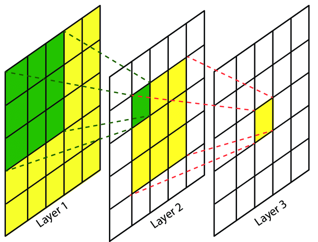] The **effective receptive field** is the part of the visual input that affects a given unit indirectly through previous convolutional layers. It grows linearly with depth. E.g., a stack of two $3 \times 3$ kernels of stride $1$ has the same effective receptive field as a single $5 \times 5$ kernel, but fewer parameters. --- exclude: true class: middle .smaller-xx.center[ ``` ---------------------------------------------------------------- Layer (type) Output Shape Param # ================================================================ Conv2d-1 [-1, 64, 224, 224] 1,792 ReLU-2 [-1, 64, 224, 224] 0 Conv2d-3 [-1, 64, 224, 224] 36,928 ReLU-4 [-1, 64, 224, 224] 0 MaxPool2d-5 [-1, 64, 112, 112] 0 Conv2d-6 [-1, 128, 112, 112] 73,856 ReLU-7 [-1, 128, 112, 112] 0 Conv2d-8 [-1, 128, 112, 112] 147,584 ReLU-9 [-1, 128, 112, 112] 0 MaxPool2d-10 [-1, 128, 56, 56] 0 Conv2d-11 [-1, 256, 56, 56] 295,168 ReLU-12 [-1, 256, 56, 56] 0 Conv2d-13 [-1, 256, 56, 56] 590,080 ReLU-14 [-1, 256, 56, 56] 0 Conv2d-15 [-1, 256, 56, 56] 590,080 ReLU-16 [-1, 256, 56, 56] 0 MaxPool2d-17 [-1, 256, 28, 28] 0 Conv2d-18 [-1, 512, 28, 28] 1,180,160 ReLU-19 [-1, 512, 28, 28] 0 Conv2d-20 [-1, 512, 28, 28] 2,359,808 ReLU-21 [-1, 512, 28, 28] 0 Conv2d-22 [-1, 512, 28, 28] 2,359,808 ReLU-23 [-1, 512, 28, 28] 0 MaxPool2d-24 [-1, 512, 14, 14] 0 Conv2d-25 [-1, 512, 14, 14] 2,359,808 ReLU-26 [-1, 512, 14, 14] 0 Conv2d-27 [-1, 512, 14, 14] 2,359,808 ReLU-28 [-1, 512, 14, 14] 0 Conv2d-29 [-1, 512, 14, 14] 2,359,808 ReLU-30 [-1, 512, 14, 14] 0 MaxPool2d-31 [-1, 512, 7, 7] 0 Linear-32 [-1, 4096] 102,764,544 ReLU-33 [-1, 4096] 0 Dropout-34 [-1, 4096] 0 Linear-35 [-1, 4096] 16,781,312 ReLU-36 [-1, 4096] 0 Dropout-37 [-1, 4096] 0 Linear-38 [-1, 1000] 4,097,000 ================================================================ Total params: 138,357,544 Trainable params: 138,357,544 Non-trainable params: 0 ---------------------------------------------------------------- Input size (MB): 0.57 Forward/backward pass size (MB): 218.59 Params size (MB): 527.79 Estimated Total Size (MB): 746.96 ---------------------------------------------------------------- ``` ] --- exclude: true class: middle .grid[ .kol-4-5[ ## GoogLeNet (Szegedy et al, 2014) Composition of two $\texttt{CONV}+\texttt{POOL}$ layers, a stack of 9 inception blocks, and a global average pooling layer. Each inception block is itself defined as a convolutional network with 4 parallel paths. .center.width-80[] .caption[Inception block] ] .kol-1-5.center[.width-100[]] ] .footnote[Credits: [Dive Into Deep Learning](https://d2l.ai/), 2020.] --- exclude: true class: middle .grid[ .kol-4-5[ ## ResNet (He et al, 2015) Composition of first layers similar to GoogLeNet, a stack of 4 residual blocks, and a global average pooling layer. Extensions consider more residual blocks, up to a total of 152 layers (ResNet-152). .center.width-80[] .center.caption[Regular ResNet block vs. ResNet block with $1\times 1$ convolution.] ] .kol-1-5[.center.width-100[]] ] .footnote[Credits: [Dive Into Deep Learning](https://d2l.ai/), 2020.] --- exclude: true class: middle Training networks of this depth is made possible because of the **skip connections** in the residual blocks. They allow the gradients to shortcut the layers and pass through without vanishing. .center.width-60[] .footnote[Credits: [Dive Into Deep Learning](https://d2l.ai/), 2020.] --- exclude: true class: middle .grid[ .kol-1-2[ .smaller-xx.center[ ``` ---------------------------------------------------------------- Layer (type) Output Shape Param # ================================================================ Conv2d-1 [-1, 64, 112, 112] 9,408 BatchNorm2d-2 [-1, 64, 112, 112] 128 ReLU-3 [-1, 64, 112, 112] 0 MaxPool2d-4 [-1, 64, 56, 56] 0 Conv2d-5 [-1, 64, 56, 56] 4,096 BatchNorm2d-6 [-1, 64, 56, 56] 128 ReLU-7 [-1, 64, 56, 56] 0 Conv2d-8 [-1, 64, 56, 56] 36,864 BatchNorm2d-9 [-1, 64, 56, 56] 128 ReLU-10 [-1, 64, 56, 56] 0 Conv2d-11 [-1, 256, 56, 56] 16,384 BatchNorm2d-12 [-1, 256, 56, 56] 512 Conv2d-13 [-1, 256, 56, 56] 16,384 BatchNorm2d-14 [-1, 256, 56, 56] 512 ReLU-15 [-1, 256, 56, 56] 0 Bottleneck-16 [-1, 256, 56, 56] 0 Conv2d-17 [-1, 64, 56, 56] 16,384 BatchNorm2d-18 [-1, 64, 56, 56] 128 ReLU-19 [-1, 64, 56, 56] 0 Conv2d-20 [-1, 64, 56, 56] 36,864 BatchNorm2d-21 [-1, 64, 56, 56] 128 ReLU-22 [-1, 64, 56, 56] 0 Conv2d-23 [-1, 256, 56, 56] 16,384 BatchNorm2d-24 [-1, 256, 56, 56] 512 ReLU-25 [-1, 256, 56, 56] 0 Bottleneck-26 [-1, 256, 56, 56] 0 Conv2d-27 [-1, 64, 56, 56] 16,384 BatchNorm2d-28 [-1, 64, 56, 56] 128 ReLU-29 [-1, 64, 56, 56] 0 Conv2d-30 [-1, 64, 56, 56] 36,864 BatchNorm2d-31 [-1, 64, 56, 56] 128 ReLU-32 [-1, 64, 56, 56] 0 Conv2d-33 [-1, 256, 56, 56] 16,384 BatchNorm2d-34 [-1, 256, 56, 56] 512 ReLU-35 [-1, 256, 56, 56] 0 Bottleneck-36 [-1, 256, 56, 56] 0 Conv2d-37 [-1, 128, 56, 56] 32,768 BatchNorm2d-38 [-1, 128, 56, 56] 256 ReLU-39 [-1, 128, 56, 56] 0 Conv2d-40 [-1, 128, 28, 28] 147,456 BatchNorm2d-41 [-1, 128, 28, 28] 256 ReLU-42 [-1, 128, 28, 28] 0 Conv2d-43 [-1, 512, 28, 28] 65,536 BatchNorm2d-44 [-1, 512, 28, 28] 1,024 Conv2d-45 [-1, 512, 28, 28] 131,072 BatchNorm2d-46 [-1, 512, 28, 28] 1,024 ReLU-47 [-1, 512, 28, 28] 0 Bottleneck-48 [-1, 512, 28, 28] 0 Conv2d-49 [-1, 128, 28, 28] 65,536 BatchNorm2d-50 [-1, 128, 28, 28] 256 ReLU-51 [-1, 128, 28, 28] 0 Conv2d-52 [-1, 128, 28, 28] 147,456 BatchNorm2d-53 [-1, 128, 28, 28] 256 ... ``` ] ] .kol-1-2[ .smaller-xx.center[ ``` ... Bottleneck-130 [-1, 1024, 14, 14] 0 Conv2d-131 [-1, 256, 14, 14] 262,144 BatchNorm2d-132 [-1, 256, 14, 14] 512 ReLU-133 [-1, 256, 14, 14] 0 Conv2d-134 [-1, 256, 14, 14] 589,824 BatchNorm2d-135 [-1, 256, 14, 14] 512 ReLU-136 [-1, 256, 14, 14] 0 Conv2d-137 [-1, 1024, 14, 14] 262,144 BatchNorm2d-138 [-1, 1024, 14, 14] 2,048 ReLU-139 [-1, 1024, 14, 14] 0 Bottleneck-140 [-1, 1024, 14, 14] 0 Conv2d-141 [-1, 512, 14, 14] 524,288 BatchNorm2d-142 [-1, 512, 14, 14] 1,024 ReLU-143 [-1, 512, 14, 14] 0 Conv2d-144 [-1, 512, 7, 7] 2,359,296 BatchNorm2d-145 [-1, 512, 7, 7] 1,024 ReLU-146 [-1, 512, 7, 7] 0 Conv2d-147 [-1, 2048, 7, 7] 1,048,576 BatchNorm2d-148 [-1, 2048, 7, 7] 4,096 Conv2d-149 [-1, 2048, 7, 7] 2,097,152 BatchNorm2d-150 [-1, 2048, 7, 7] 4,096 ReLU-151 [-1, 2048, 7, 7] 0 Bottleneck-152 [-1, 2048, 7, 7] 0 Conv2d-153 [-1, 512, 7, 7] 1,048,576 BatchNorm2d-154 [-1, 512, 7, 7] 1,024 ReLU-155 [-1, 512, 7, 7] 0 Conv2d-156 [-1, 512, 7, 7] 2,359,296 BatchNorm2d-157 [-1, 512, 7, 7] 1,024 ReLU-158 [-1, 512, 7, 7] 0 Conv2d-159 [-1, 2048, 7, 7] 1,048,576 BatchNorm2d-160 [-1, 2048, 7, 7] 4,096 ReLU-161 [-1, 2048, 7, 7] 0 Bottleneck-162 [-1, 2048, 7, 7] 0 Conv2d-163 [-1, 512, 7, 7] 1,048,576 BatchNorm2d-164 [-1, 512, 7, 7] 1,024 ReLU-165 [-1, 512, 7, 7] 0 Conv2d-166 [-1, 512, 7, 7] 2,359,296 BatchNorm2d-167 [-1, 512, 7, 7] 1,024 ReLU-168 [-1, 512, 7, 7] 0 Conv2d-169 [-1, 2048, 7, 7] 1,048,576 BatchNorm2d-170 [-1, 2048, 7, 7] 4,096 ReLU-171 [-1, 2048, 7, 7] 0 Bottleneck-172 [-1, 2048, 7, 7] 0 AvgPool2d-173 [-1, 2048, 1, 1] 0 Linear-174 [-1, 1000] 2,049,000 ================================================================ Total params: 25,557,032 Trainable params: 25,557,032 Non-trainable params: 0 ---------------------------------------------------------------- Input size (MB): 0.57 Forward/backward pass size (MB): 286.56 Params size (MB): 97.49 Estimated Total Size (MB): 384.62 ---------------------------------------------------------------- ``` ] ] ] --- class: middle ## The benefits of depth .center.width-100[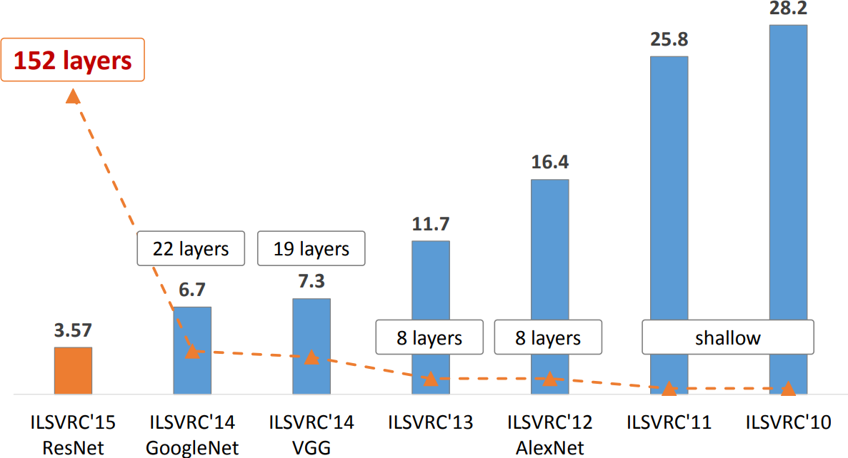] --- name: ex3 # .red[Exercise 3] Your task is to code up a simple convolutional network and train it to perform parameter regression. Goal is to estimat the radius (and position?) of a partially visible ring. .center[ 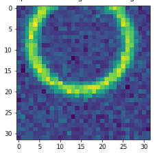 ] - Start with this [Google Colab](https://colab.research.google.com/drive/1uWnYd8KuizlbqemCPrSZD6hmxhF-2dSM) notebook. - Use a structure $\texttt{INPUT} \to [\texttt{CONV} \to \texttt{RELU} \to \texttt{POOL}]\texttt{\*2} \to \texttt{FC} \to \texttt{RELU} \to \texttt{FC}$, which is similar to the LeNet structure. --- class: middle, center .center[] --- class: middle # Under the hood --- class: middle Understanding what is happening in deep neural networks after training is complex and the tools we have are limited. In the case of convolutional neural networks, we can look at: - the network's kernels as images - internal activations on a single sample as images - distributions of activations on a population of samples - derivatives of the response with respect to the input - maximum-response synthetic samples .footnote[Credits: Francois Fleuret, [EE559 Deep Learning](https://fleuret.org/ee559/), EPFL.] --- # Looking at filters <br><br><br><br><br> LeNet's first convolutional layer, all filters. .width-100[] .footnote[Credits: Francois Fleuret, [EE559 Deep Learning](https://fleuret.org/ee559/), EPFL.] --- class: middle LeNet's second convolutional layer, first 32 filters. .center.width-70[] .footnote[Credits: Francois Fleuret, [EE559 Deep Learning](https://fleuret.org/ee559/), EPFL.] --- class: middle AlexNet's first convolutional layer, first 20 filters. .center.width-100[] .footnote[Credits: Francois Fleuret, [EE559 Deep Learning](https://fleuret.org/ee559/), EPFL.] --- # Maximum response samples Convolutional networks can be inspected by looking for synthetic input images $\mathbf{x}$ that maximize the activation $\mathbf{h}\_{\ell,d}(\mathbf{x})$ of a chosen convolutional kernel $\mathbf{u}$ at layer $\ell$ and index $d$ in the layer filter bank. These samples can be found by gradient ascent on the input space: $$\begin{aligned} \mathcal{L}\_{\ell,d}(\mathbf{x}) &= ||\mathbf{h}\_{\ell,d}(\mathbf{x})||\_2\\\\ \mathbf{x}\_0 &\sim U[0,1]^{C \times H \times W } \\\\ \mathbf{x}\_{t+1} &= \mathbf{x}\_t + \gamma \nabla\_{\mathbf{x}} \mathcal{L}\_{\ell,d}(\mathbf{x}\_t) \end{aligned}$$ --- class: middle .width-100[] .center[VGG-16, convolutional layer 1-1, a few of the 64 filters] .footnote[Credits: Francois Chollet, [How convolutional neural networks see the world](https://blog.keras.io/how-convolutional-neural-networks-see-the-world.html), 2016.] --- class: middle .width-100[] .center[VGG-16, convolutional layer 2-1, a few of the 128 filters] .footnote[Credits: Francois Chollet, [How convolutional neural networks see the world](https://blog.keras.io/how-convolutional-neural-networks-see-the-world.html), 2016.] --- class: middle .width-100[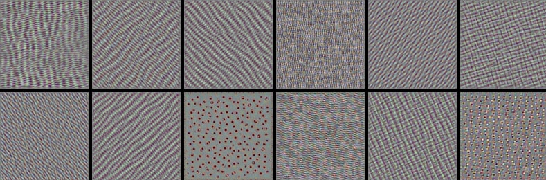] .center[VGG-16, convolutional layer 3-1, a few of the 256 filters] .footnote[Credits: Francois Chollet, [How convolutional neural networks see the world](https://blog.keras.io/how-convolutional-neural-networks-see-the-world.html), 2016.] --- class: middle .width-100[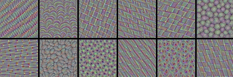] .center[VGG-16, convolutional layer 4-1, a few of the 512 filters] .footnote[Credits: Francois Chollet, [How convolutional neural networks see the world](https://blog.keras.io/how-convolutional-neural-networks-see-the-world.html), 2016.] --- class: middle .width-100[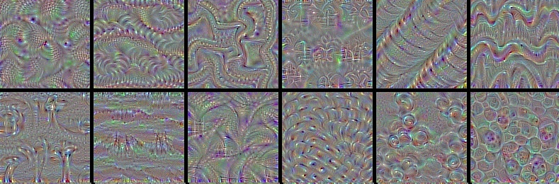] .center[VGG-16, convolutional layer 5-1, a few of the 512 filters] .footnote[Credits: Francois Chollet, [How convolutional neural networks see the world](https://blog.keras.io/how-convolutional-neural-networks-see-the-world.html), 2016.] --- class: middle Some observations: - The first layers appear to encode direction and color. - The direction and color filters get combined into grid and spot textures. - These textures gradually get combined into increasingly complex patterns. The network appears to learn a .bold[hierarchical composition of patterns]. .width-70.center[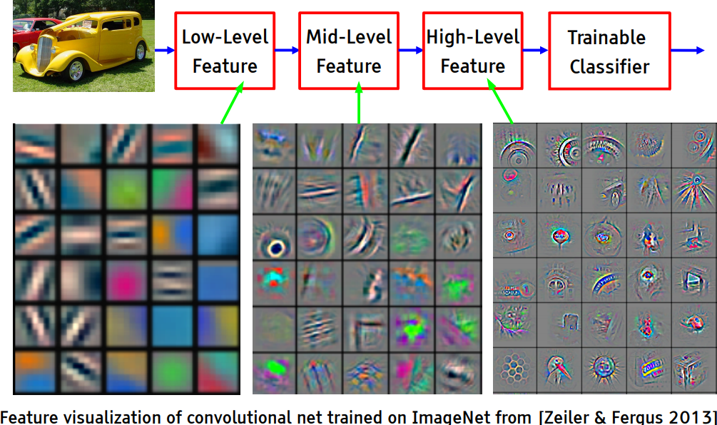] --- <br><br><br> What if we build images that maximize the activation of a chosen class output? -- count: false The left image is predicted **with 99.9% confidence** as a magpie! .grid[ .kol-1-2.center[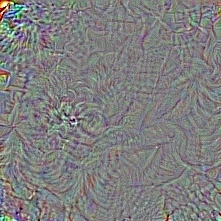] .kol-1-2.center[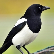] ] .footnote[Credits: Francois Chollet, [How convolutional neural networks see the world](https://blog.keras.io/how-convolutional-neural-networks-see-the-world.html), 2016.] --- class: middle, black-slide .center[ <iframe width="600" height="400" src="https://www.youtube.com/embed/SCE-QeDfXtA?&loop=1&start=0" frameborder="0" volume="0" allowfullscreen></iframe> ] .bold[Deep Dream.] Start from an image $\mathbf{x}\_t$, offset by a random jitter, enhance some layer activation at multiple scales, zoom in, repeat on the produced image $\mathbf{x}\_{t+1}$. --- # Biological plausibility .center.width-80[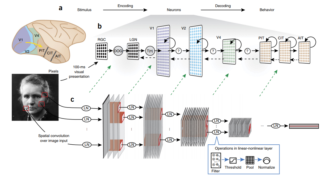] .italic["Deep hierarchical neural networks are beginning to transform neuroscientists’ ability to produce quantitatively accurate computational models of the sensory systems, especially in higher cortical areas where neural response properties had previously been enigmatic."] .footnote[Credits: Yamins et al, Using goal-driven deep learning models to understand sensory cortex, 2016.] --- class: middle, center # Neural likelihood free inference --- class: middle # Bayes theorem Bayes theorem connects likelihood, prior, posterior and evidence $$ P(\theta|x) = \frac{P(x|\theta) P(\theta)}{P(x)} $$ --- class: center, middle, black-slide <iframe width="600" height="450" src="https://www.youtube.com/embed/Kq7e6cj2nDw" frameborder="0" allowfullscreen></iframe> --- # The likelihood-to-evidence ratio In order to evaluate the probability of any outcome, we have to sum or integrate over all possible paths that could have led to this outcome $$ P(x|\theta) = \underbrace{\int dz}_\text{\color{red} intractable} \delta(x - z(t)) P(z|\theta) $$ -- count: false Even if we could estimate the shape of $P(x|\theta)$ for paths that lead to some actually observed values of $x$, in order to get the normalization of $P(x)$ we have to know also all paths $z$ that do __not__ lead to $x$. -- count: false It turns out that often the likelihood **ratios** are easier to estimate, since normalizing factors drop out. One particular combination is the .bold[likelihood-to-evidence ratio]: $$ r(x, \theta) \equiv \frac{P(x|\theta)}{P(x)} $$ .bold[Goal]: Train a neural network to approximate $r(x, \theta)$. ??? Calculating the likelihood is often .red[untractable], due to large number of internal parameters $$ P(x|\theta) = \underbrace{\int \int dz\, dy}_\text{\color{red} untractable} \, P(x|z, y, \theta) P(z|y) P(y) P(\theta) $$ --- # Neural likelihood-free inference .bold[Starting point]: for any pair of observation $x$ and model parameter $\theta$, the goal is to estimate the probability that this pair belongs one of the following classes: .grid[ .kol-1-2[ $H_0$: Data $x$ comes from model $\theta$ $H_1$: Data $x$ and model $\theta$ are unrelated ] .kol-1-2[ $(x, \theta) \sim P(x, \theta) = P(x|\theta)P(\theta)$ $(x, \theta) \sim P(x)P(\theta)$ ] ] .red[Note]: The likelihood ratio for these two hypothesis is our function of interest, $r(x, \theta)$. --- # Loss function .bold[Strategy:] We train a neural network $d_\phi(x, \theta)$ as binary classifier to estimate the probability of hypothesis $H_0$ ($y=0$) or $H_1$ ($y=1$). The corresponding loss function (see logistic regression example) is $$ L\left[d(x, \theta)\right] = \int dx d\theta \left[ p(x, \theta) \ln\left(d(x, \theta)\right) + p(x)p(\theta) \ln\left(1-d(x, \theta)\right) \right] $$ -- count: false Minimizing that function yields $$ d(x, \theta) = \frac{P(x, \theta)}{P(x, \theta) + P(x)P(\theta)} $$ -- count: false It is easy to see that the likelihood-to-evidence ratio is then given by $$ r(x,\theta) \equiv \frac{P(x|\theta)}{P(x)} = \frac{1}{d(x, \theta)}-1. $$ --- name: ex4 # .red[Exercise 4: Neural posterior estimation] Your task is to take the solution to [exercise 3](#ex3) and replace point estimation with posterior estimation. To this end you have to - Adopt the convolutional neural network such that it takes an additional input, the radius $r$, and such that the output is between zero and one. A good way to do that is to replace the last layer with .center[$\texttt{(INPUT, r)} \to \texttt{FC} \to \texttt{RELU} \to \texttt{FC} \to \texttt{SIGMOID}\to\texttt{OUTPUT}$] Here, $\texttt{INPUT}$ is the output of the second-to-last $\texttt{FC}$, which is concatenated with the input variable $r$. - Replace the loss function by the above binary cross-entropy loss function $L[d(x, \theta)]$. Once this is done - Train the network and show that the posterior (which is $\propto \exp(-r(x, \theta))$), peaks usually close to the true value - Explore how the posterior becomes broaders when making the signal model more complicated (e.g. by masking random regions). --- class: end-slide, center count: false The end. --- count: false # References - Francois Fleuret, Deep Learning Course, [4.4. Convolutions](https://fleuret.org/ee559/ee559-slides-4-4-convolutions.pdf), EPFL, 2018. - Yannis Avrithis, Deep Learning for Vision, [Lecture 1: Introduction](https://sif-dlv.github.io/slides/intro.pdf), University of Rennes 1, 2018. - Yannis Avrithis, Deep Learning for Vision, [Lecture 7: Convolution and network architectures ](https://sif-dlv.github.io/slides/conv.pdf), University of Rennes 1, 2018. - Olivier Grisel and Charles Ollion, Deep Learning, [Lecture 4: Convolutional Neural Networks for Image Classification ](https://m2dsupsdlclass.github.io/lectures-labs/slides/04_conv_nets/index.html#1), Université Paris-Saclay, 2018. - Rosenblatt, F. (1958). The perceptron: a probabilistic model for information storage and organization in the brain. Psychological review, 65(6), 386. - Bottou, L., & Bousquet, O. (2008). The tradeoffs of large scale learning. In Advances in neural information processing systems (pp. 161-168). - Rumelhart, D. E., Hinton, G. E., & Williams, R. J. (1986). Learning representations by back-propagating errors. nature, 323(6088), 533.