Machine Learning for Physics and Astronomy
Christoph Weniger
Thursday, 3 March 2022
Chapter 1: Classification
Motivation
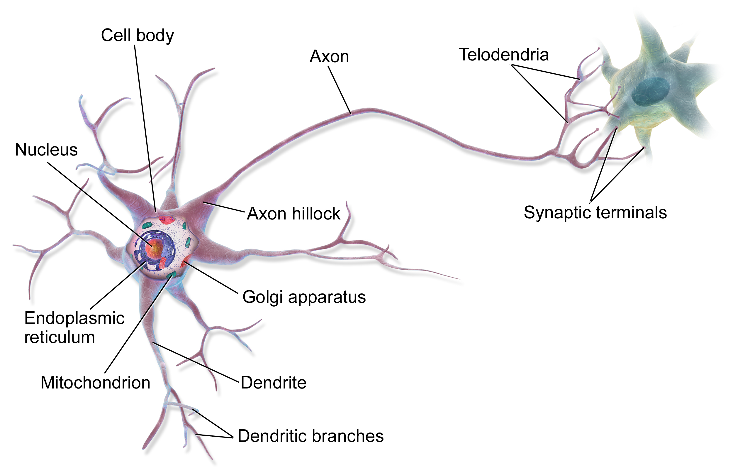
During this chapter we will lay the groundwork for studying deep neural networks lated in the course. What we will discuss here is in fact the mathematics of a single artifical neuron.
![]()
(biological neuron)
Classification Concepts
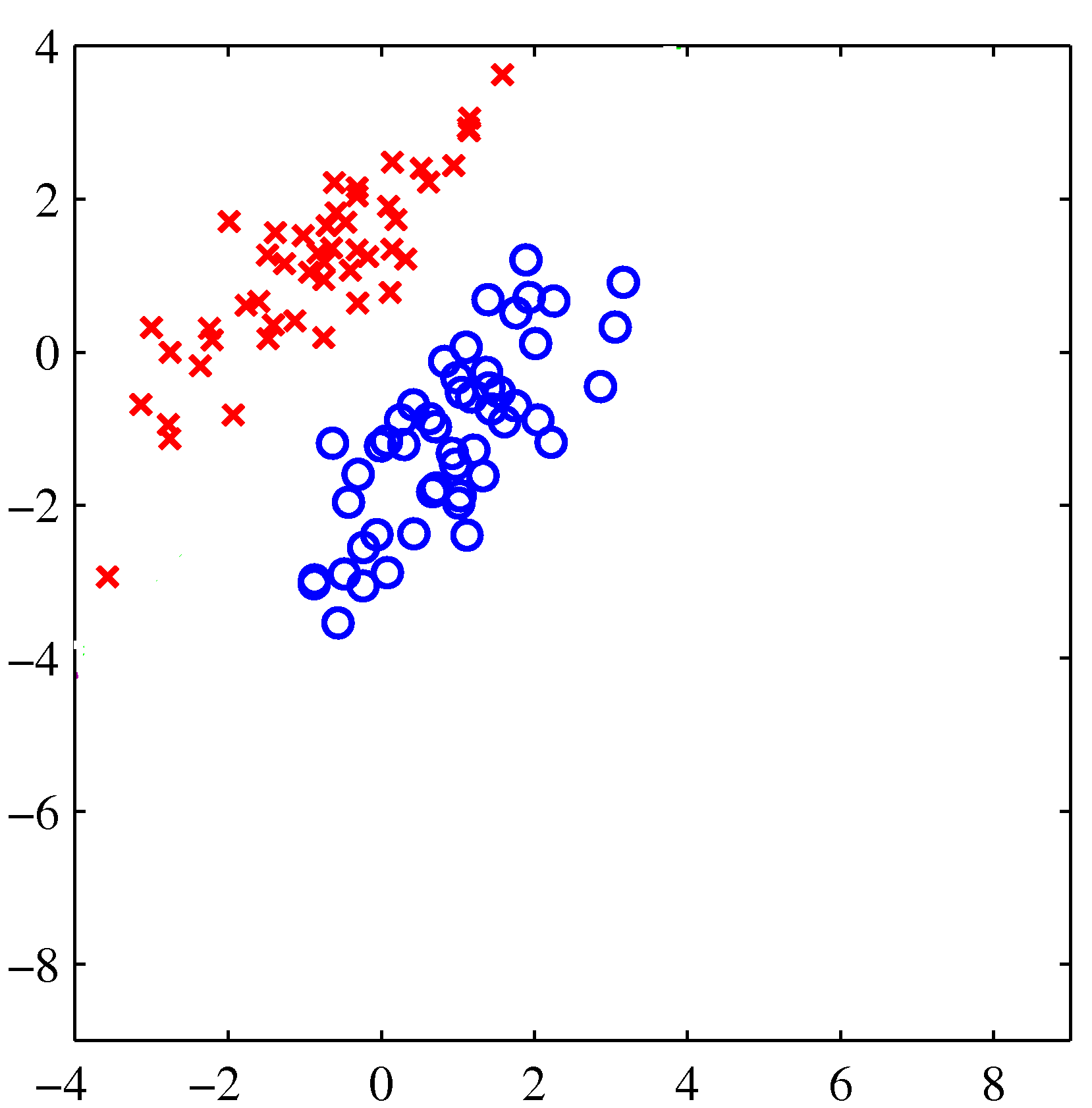
Consider a dataset that is described by two real values and has two possible class labels (red and blue).
Image Credit: PRML: C. Bishop, Fig. 4.4
Classification Concepts
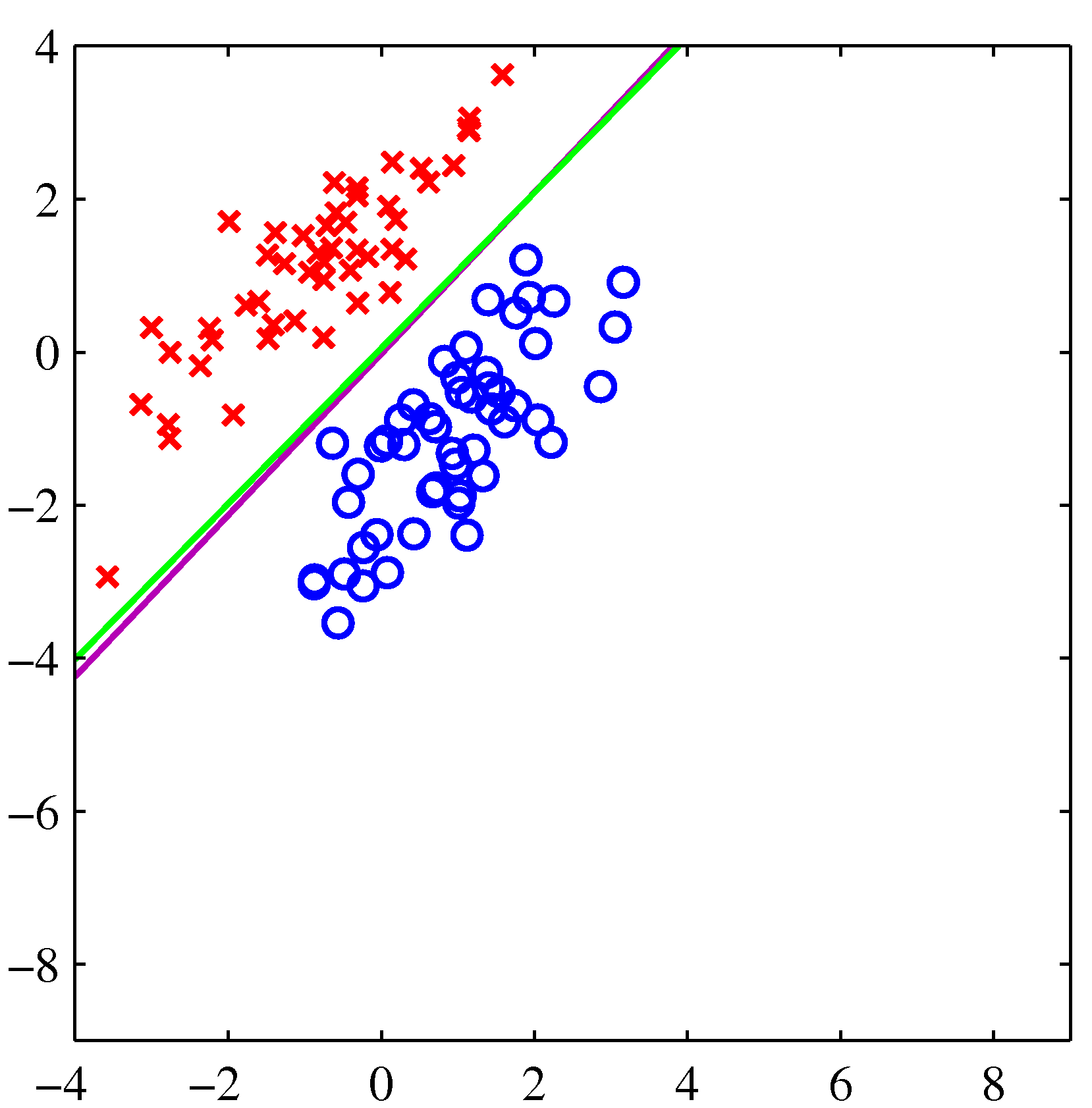
Visually, we can see that the dataset is separable, and more specifically linearly separable because we can draw a boundary, and more specifically a line, between the two classes without having misclassified data points.
Image Credit: PRML: C. Bishop, Fig. 4.4
Naive Classification
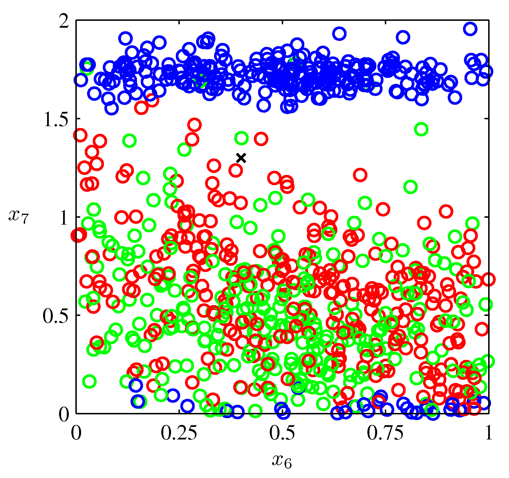
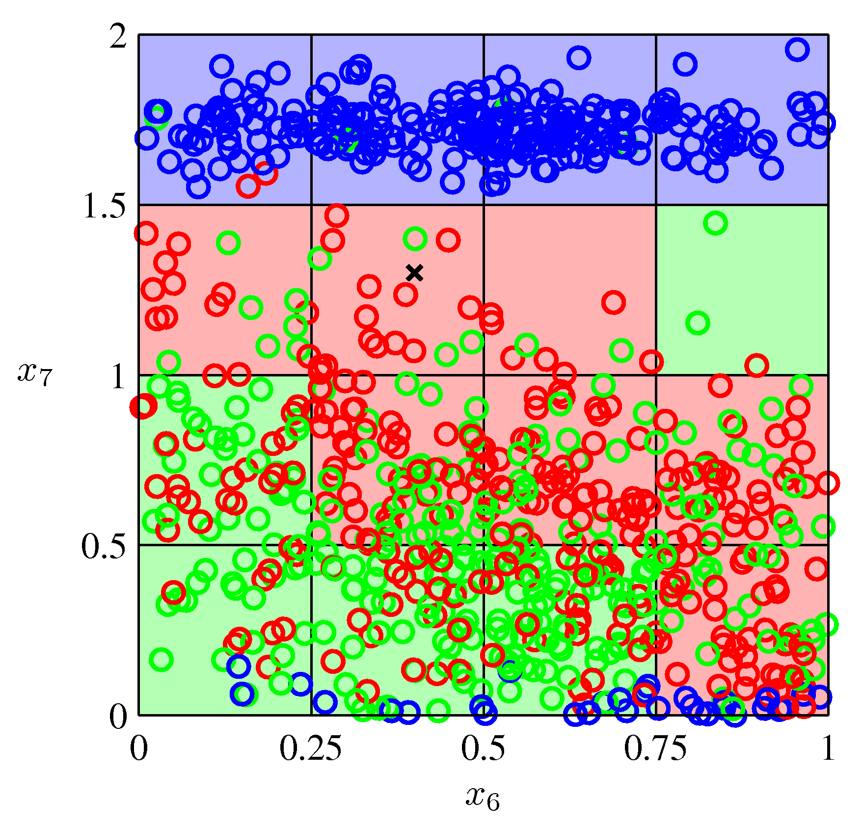
Most datasets, however, are not so simple. How could we model this data such that given a new point, we could predict its label (red, green, or blue)?
Image Credit: PRML: C. Bishop, Fig. 1.19
Naive Classification
One very simple approach would be to divide the input space into regularly sized cells and assign any new data point the label that a majority of the training points in the cell have.
Image Credit: PRML: C. Bishop, Fig. 1.20
Logistic Regression
A probabilistic classification method
Analogy with a single neuron
The linear case has a nice interpretation in terms of a single neuron.
- The synapses weight input signal with weights \(\mathbf{w}\)
- The neuron sums it all up and fires if input is above some threshold
\[
y(\mathbf{x}) = f(\mathbf{w}^T \mathbf{x} + w_0)
\]
![]()
(the analogy would be even better if we were to use a step function as activation function)
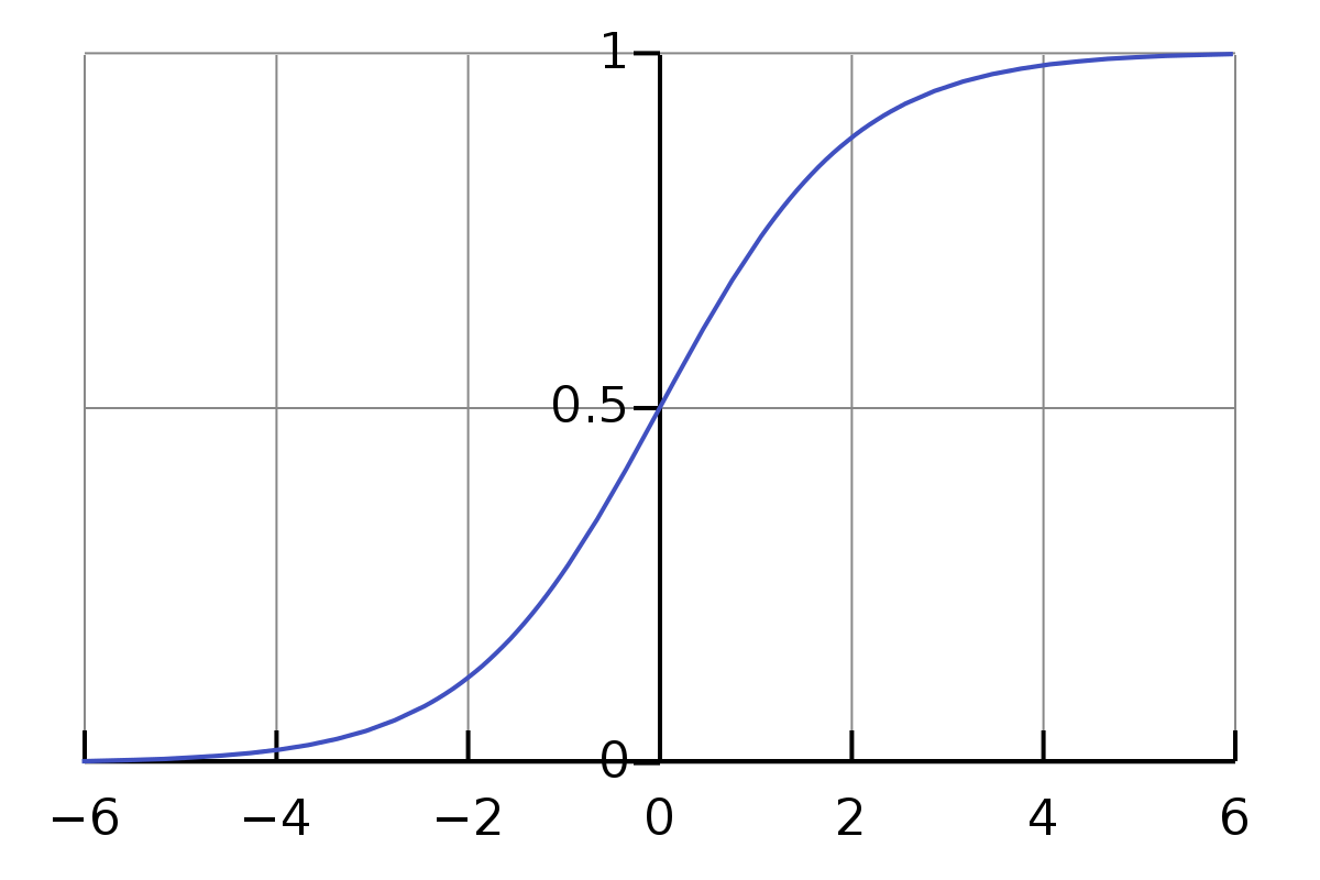
Sigmoid
For classification, the most important activation function is the logistic sigmoid function (from now on simply sigmoid), which maps the whole real number range to the finite interval (0,1).
\[\sigma(x) = \frac{1}{1+\exp(-x)}\]
Sigmoid also satisfies the useful symmetry property: \(\sigma(-x) = 1 - \sigma(x)\).
Logistic regression
Like in the case of linear regression, we can drastically increase the expressivity of the model by using basis functions \(\phi_i(\mathbf{x})\). In that case the model becomes
\[
y(\mathbf{x}) = f(\mathbf{w}^T \boldsymbol{\phi}(\mathbf{x}) + w_0)
\]
Logistic Regression
For a dataset \({\boldsymbol{\phi}_n, t_n}\) where \(t_n = 0, 1\) and \(\boldsymbol{\phi}_n = \boldsymbol{\phi} (\mathbf{x}_n)\) with \(n = 1, \ldots , N\), we write the likelihood as \[
p(\mathtt{t} | \mathbf{w}) = \prod^N_{n=1} y_n^{t_n} \{ 1 - y_n \}^{1-t_n}
\] where \(\mathtt{t} = (t_1, \ldots , t_N)^T\) and \(y_n = p(C_1 | \boldsymbol{\phi}_n) = \sigma (\mathbf{w}^T \boldsymbol{\phi}_n)\)
As per usual, we can define an error function by taking the negative log-likelihood, which gives us the cross-entropy error function in the form
\[
E(\mathbf{w}) = -\ln p(\mathtt{t}|\mathbf{w}) = -\sum^N_{n=1} \{ t_n \ln y_n + (1- t_n)\ln (1-y_n) \}
\]
Logistic Regression
Although we have defined an error function, there is no closed solution for the optimal parameters \(\mathbf{w}\). We will therefore now be exploring gradient descent algorithms for optimization. For this, we will need the gradient of the error function with respect to the parameters \(\mathbf{w}\) :
\[
\nabla_{\mathbf{w}} E(\mathbf{w}) = \sum^N_{n=1} (y_n - t_n)\boldsymbol{\phi}_n
\]
Gradient Descent
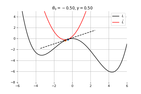
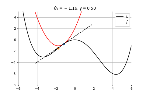
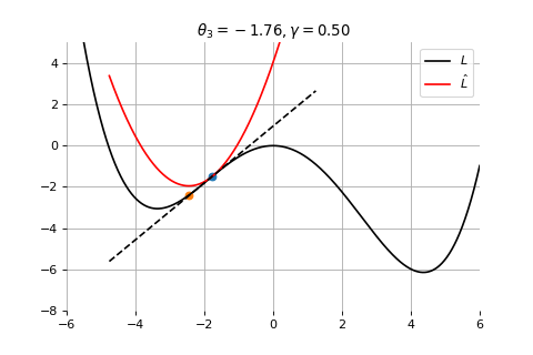
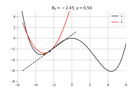
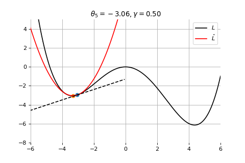
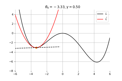
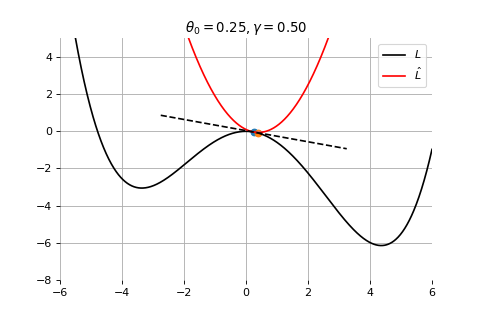
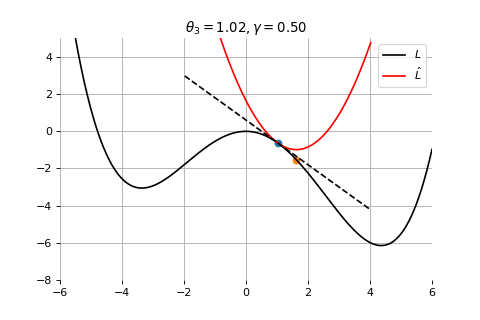
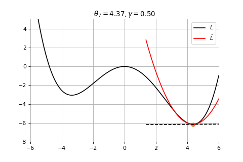
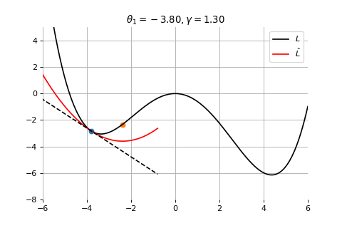
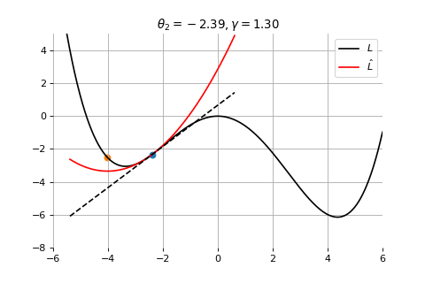
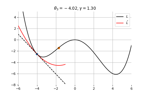
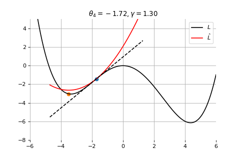
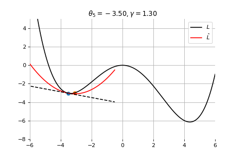
To minimize the error function \(E(\theta)\) defined over model parameters \(\theta\) (e.g. \(\mathbf{w}\) and \(b\)), the simplest gradient method of gradient descent uses local linear information to iteratively move towards a local minimum. The algorithm must be initialized with an initial value of parameters \(\theta_0\). A first order approximation to \(E(\theta)\) around \(\theta_0\) can be given as
\[
\hat{E}(\epsilon ; \theta_0) = E(\theta_0) + \epsilon^T \nabla E(\theta_0) + \frac{1}{2\gamma}||\epsilon||^2
\]
Gradient Descent
We can minimize the approximation \(\hat{E}({\theta }_0)\) in the usual way:
\[
\begin{aligned}
\nabla_\epsilon \hat{E}(\epsilon ; \theta_0) &= 0 \\
&= \nabla_\theta E(\theta_0) + \frac{1}{\gamma}\epsilon
\end{aligned}
\] which results in the best improvement when \(\epsilon = -\gamma \nabla_\theta E(\theta_0)\).
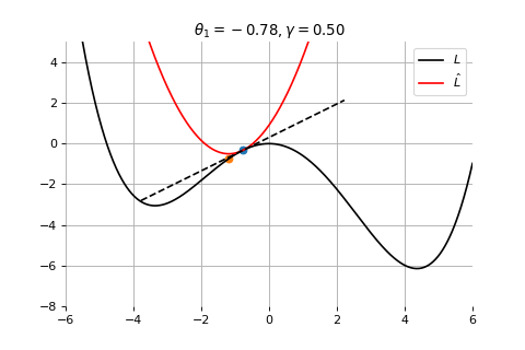
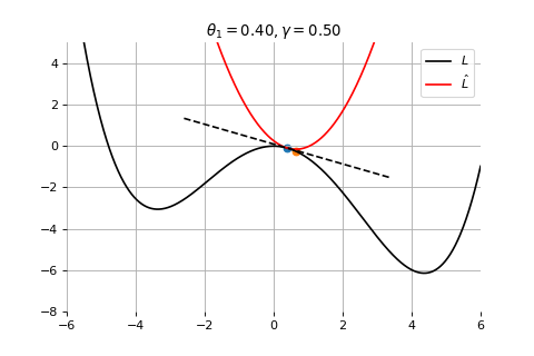
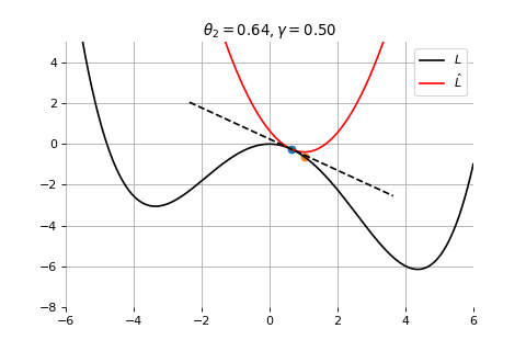
Therefore model parameters can be updated iteratively using the update rule \[
\theta_{t+1} = \theta_{t} -\gamma \nabla_\theta E(\theta_t)
\]
where - \(\theta_0\) are the initial conditions of the parameters of the model - \(\gamma\) is known as the learning rate - choosing both correctly is critical for the convergence of the update rule
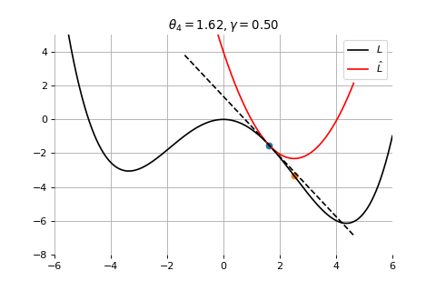
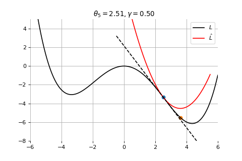
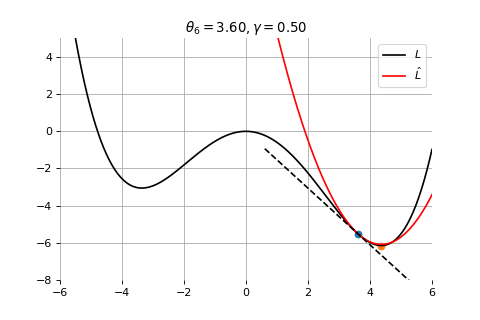
Example 1: Convergence to a local minima
Example 2: Convergence to the global minima
Example 3: Divergence due to a too large learning rate
(Batch) Gradient Descent
For logistic regression, as well as for most error functions, the error function \(E\), as well as its derivative is defined as a sum over all data points
\[
\begin{aligned}
E(\mathbf{w}) &= -\ln p(\mathtt{t}|\mathbf{w}) = -\sum^N_{n=1} \{ t_n \ln y_n + (1- t_n)\ln (1-y_n) \} \\
\nabla E(\mathbf{w}) &= \sum^N_{n=1} (y_n - t_n)\boldsymbol{\phi}_n
\end{aligned}
\]
To find the full gradient, we need to therefore look at every data point. Because of this, regular gradient descent is often referred to as batch gradient descent. However, the complexity of an update step grows linearly (!) with the size of the dataset. This is not good.
Stochastic Gradient Descent
Since we are optimizing already an approximation, it should not be necessary to carry out the minimization to great accuracy. Therefore we often use stochastic gradient descent for an update rule:
\[
\theta_{t+1} = \theta_{t} -\gamma \nabla_\theta e(y_{i(t+1)}, f(\mathbf{x}_{i(t+1)},\theta_t))
\]
- \(e(y_{i(t+1)}, f(\mathbf{x}_{i(t+1)},\theta_t))\) is the error of example \(i\)
- iteration complexity is independent of \(N\)
- the stochastic process refers to the fact that the examples \(i\) are picked randomly at each iteration
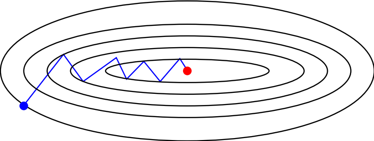
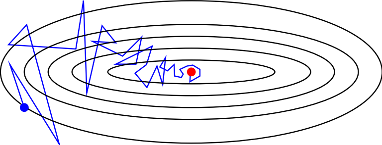
Stochastic vs batch gradient descent
![]()
Batch gradient descent
![]()
Stochastic gradient descent
Why is stochastic gradient descent still a good idea?
- Informally, averaging the update \[
\theta_{t+1} = \theta_{t} -\gamma \nabla_\theta e(y_{i(t+1)}, f(\mathbf{x}_{i(t+1)},\theta_t))
\] over all choices \(i(t+1)\) restores batch gradient descent.
- Formally, if the gradient estimate is unbiased, e.g., if \[
\begin{aligned}
\mathbb{E}_{i(t+1)}[\nabla e(y_{i(t+1)}, f(\mathbf{x}_{i(t+1)}; \theta_t))] &= \frac{1}{N} \sum_{\mathbf{x}_i, y_i \in \mathbf{d}} \nabla e(y_i, f(\mathbf{x}_i; \theta_t)) \\
&= \nabla E(\theta_t)
\end{aligned}
\] then the formal convergence of SGD can be proven, under appropriate assumptions.
Exercises
![]()
shorturl.at/frCLX