Machine Learning for Physics and Astronomy
Thursday, 3 March 2022
A story of three activation functions
In this lecture I will discuss the role of various activation functions. We will construct a dense deep neural networks, also known as multi layer percetrons.
 Sign
Sign
 Sigmoid
 ReLU
ReLU
1) The sign activation function
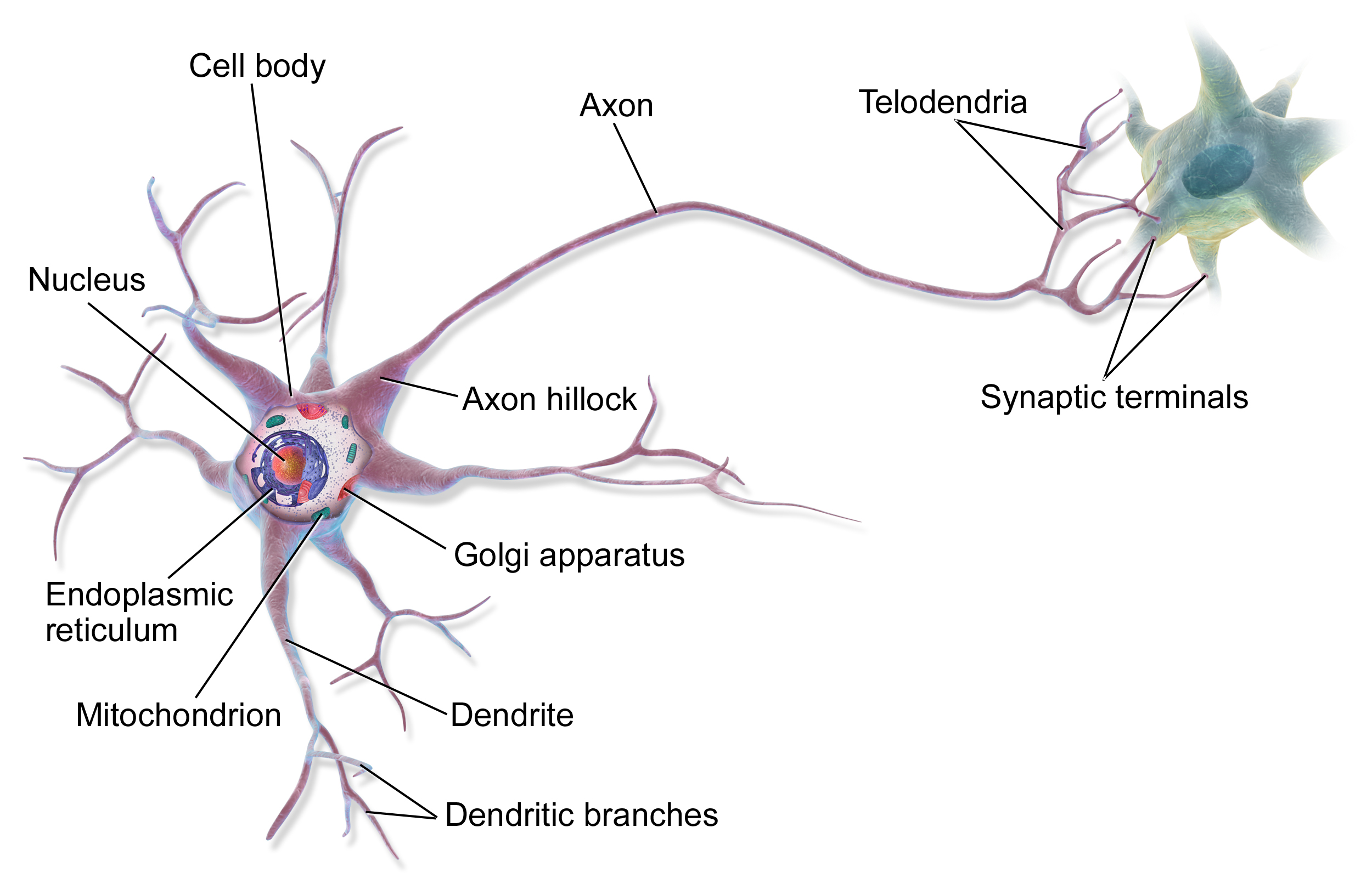
Perceptron
The perceptron model (Rosenblatt, 1957)
\[f(\mathbf{x}) = \begin{cases} 1 &\text{if } \sum_i w_i x_i + b \geq 0 \\ 0 &\text{otherwise} \end{cases}\]
was originally motivated by biology, with \(w_i\) being synaptic weights and \(x_i\) and \(f\) firing rates.
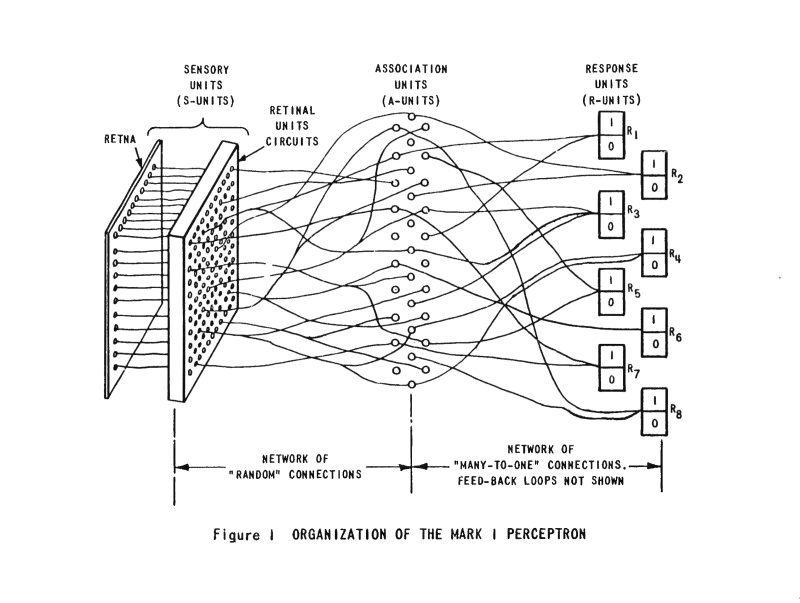
Credits: Frank Rosenblatt, Mark I Perceptron operators’ manual, 1960.
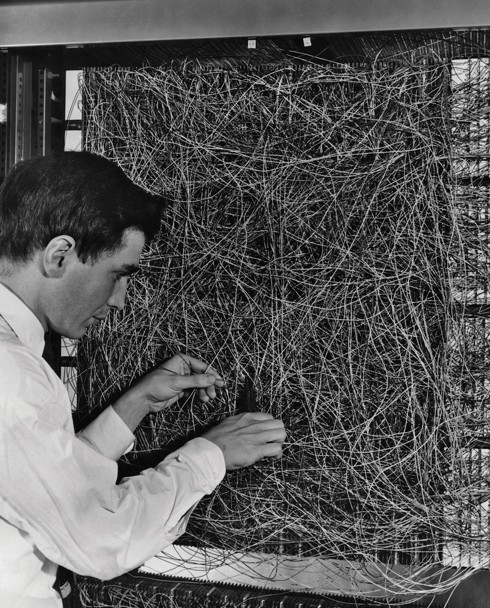
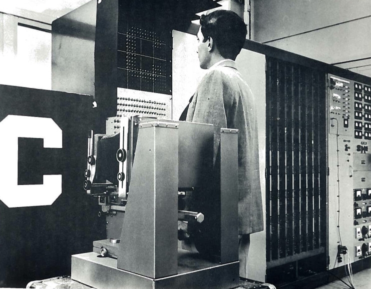
The Mark I Percetron (Frank Rosenblatt).
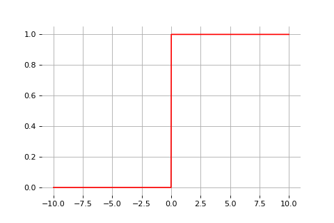
Binary step activation function
Let us define the (non-linear) activation function:
\[\text{sign}(x) = \begin{cases} 1 &\text{if } x \geq 0 \\ 0 &\text{otherwise} \end{cases}\]
The perceptron classification rule can be rewritten as \[f(\mathbf{x}) = \text{sign}(\sum_i w_i x_i + b).\]
Computational graphs

The computation of \[f(\mathbf{x}) = \text{sign}(\sum_i w_i x_i + b)\] can be represented as a computational graph where
- white nodes correspond to inputs and outputs;
- red nodes correspond to model parameters;
- blue nodes correspond to intermediate operations.
Computational graphs
In terms of tensor operations, \(f\) can be rewritten as \[f(\mathbf{x}) = \text{sign}(\mathbf{w}^T \mathbf{x} + b),\] for which the corresponding computational graph of \(f\) is:

2) The sigmoid activation function
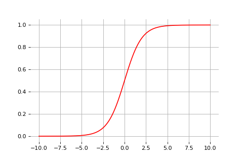
The sigmoid function
Extending binary logic with Bayesian probabilities motivates the sigmoid function, \[\sigma(x) = \frac{1}{1 + \exp(-x)}\] which looks like a soft heavyside.
Therefore, an overall model \(f(\mathbf{x};\mathbf{w},b) = \sigma(\mathbf{w}^T \mathbf{x} + b)\) is very similar to the perceptron.

This unit (or variants with other activation functions, see below) is the main primitive of all neural networks!
Recap: Logistic regression
(we discussed this already in the classification chapter)
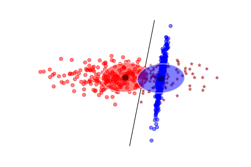
Consider the model \[P(Y=1|\mathbf{x}) = \sigma\left(\mathbf{w}^T \mathbf{x} + b\right)\].
- colored classes correspond to \(Y=1\) and \(Y=0\)
- no model assumptions on class population (Gaussian class populations, homoscedasticity);
- goal: instead, find \(\mathbf{w}, b\) that maximizes the likelihood of the data.
Multi-layer perceptron
So far we considered the logistic unit \(h=\sigma\left(\mathbf{w}^T \mathbf{x} + b\right)\), where \(h \in \mathbb{R}\), \(\mathbf{x} \in \mathbb{R}^p\), \(\mathbf{w} \in \mathbb{R}^p\) and \(b \in \mathbb{R}\).
These units can be composed in parallel to form a layer with \(q\) outputs: \[\mathbf{h} = \sigma(\mathbf{W}^T \mathbf{x} + \mathbf{b})\] where \(\mathbf{h} \in \mathbb{R}^q\), \(\mathbf{x} \in \mathbb{R}^p\), \(\mathbf{W} \in \mathbb{R}^{p\times q}\), \(b \in \mathbb{R}^q\) and where \(\sigma(\cdot)\) is upgraded to the element-wise sigmoid function.


In the forward pass, intermediate values are all computed from inputs to outputs, which results in the annotated computational graph below:


Let us zoom in on the computation of the network output \(\hat{y}\) and of its derivative with respect to \(\mathbf{W}_1\).
- Forward pass: values \(u_1\), \(u_2\), \(u_3\) and \(\hat{y}\) are computed by traversing the graph from inputs to outputs given \(\mathbf{x}\), \(\mathbf{W}_1\) and \(\mathbf{W}_2\).
- Backward pass: by the chain rule we have \[\begin{aligned} \frac{\text{d} \hat{y}}{\text{d} \mathbf{W}_1} &= \frac{\partial \hat{y}}{\partial u_3} \frac{\partial u_3}{\partial u_2} \frac{\partial u_2}{\partial u_1} \frac{\partial u_1}{\partial \mathbf{W}_1} \\ &= \frac{\partial \sigma(u_3)}{\partial u_3} \frac{\partial \mathbf{W}_2^T u_2}{\partial u_2} \frac{\partial \sigma(u_1)}{\partial u_1} \frac{\partial \mathbf{W}_1^T \mathbf{x}}{\partial \mathbf{W}_1} \end{aligned}\] Note how evaluating the partial derivatives requires the intermediate values computed forward.
The vanishing gradients problem
Training deep MLPs with many layers has for long (pre-2011) been very difficult due to the vanishing gradient problem.
- Small gradients slow down, and eventually block, stochastic gradient descent.
- This results in a limited capacity of learning.
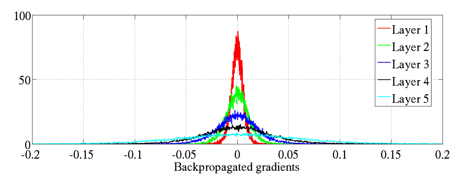
Backpropagated gradients normalized histograms (Glorot and Bengio, 2010).
Gradients for layers far from the output vanish to zero.
3) The ReLU activation function
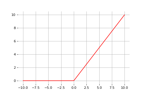
Rectified linear units
Instead of the sigmoid activation function, modern neural networks are mostly based on rectified linear units (ReLU) (Glorot et al, 2011):
\[\text{ReLU}(x) = \max(0, x)\]
Note that the derivative of the ReLU function is
\[\frac{\text{d}}{\text{d}x} \text{ReLU}(x) = \begin{cases}
0 &\text{if } x \leq 0 \\
1 &\text{otherwise}
\end{cases}\] 
For \(x=0\), the derivative is undefined. In practice, it is set to zero.
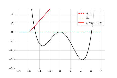
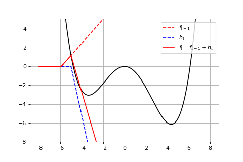
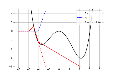
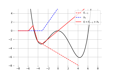
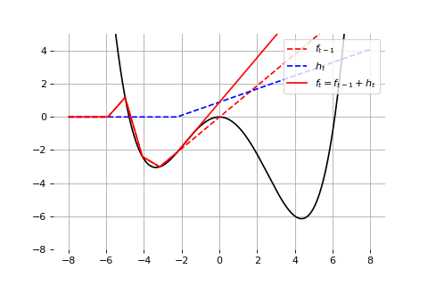
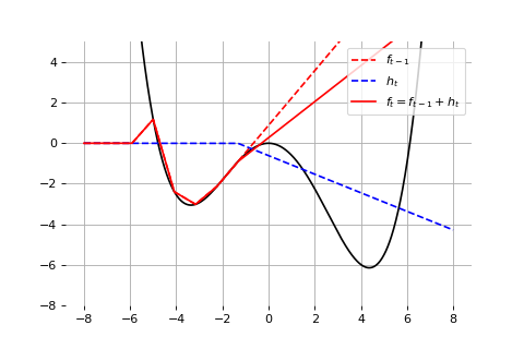
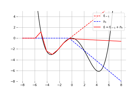
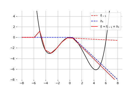
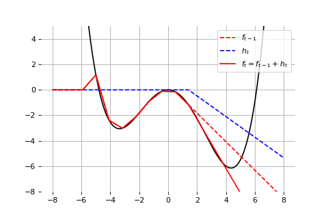
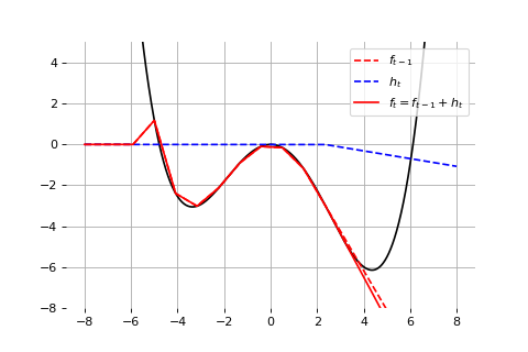
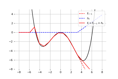
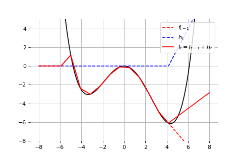
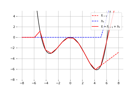
Example: Universal approximation
Exercises

shorturl.at/yBW16