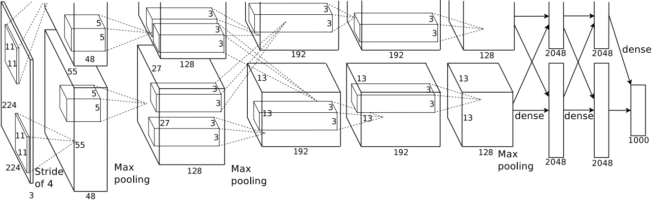
Krizhevsky trains a convolutional network on ImageNet with two GPUs.
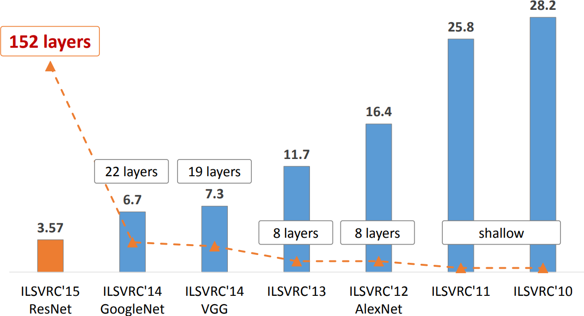
16.4% top-5 error on ILSVRC’12, outperforming all other entries by 10% or more.
This event triggers the deep learning revolution.
Convolutions
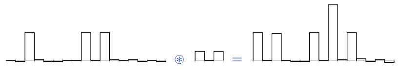
For one-dimensional tensors, given an input vector \(\mathbf{x} \in \mathbb{R}^W\) and a convolutional kernel \(\mathbf{u} \in \mathbb{R}^w\), the discrete convolution\(\mathbf{x} \circledast \mathbf{u}\) is a vector of size \(W - w + 1\) such that \[\begin{aligned}
(\mathbf{x} \circledast \mathbf{u})[i] &= \sum_{m=0}^{w-1} x_{m+i} u_m .
\end{aligned}
\]
Note: Technically, \(\circledast\) denotes the cross-correlation operator. However, most machine learning libraries call it convolution.
Convolutions generalize to multi-dimensional tensors:
In its most usual form, a convolution takes as input a 3D tensor \(\mathbf{x} \in \mathbb{R}^{C \times H \times W}\), called the input feature map.
A kernel \(\mathbf{u} \in \mathbb{R}^{C \times h \times w}\) slides across the input feature map, along its height and width. The size \(h \times w\) is the size of the receptive field.
At each location, the element-wise product between the kernel and the input elements it overlaps is computed and the results are summed up.
The final output \(\mathbf{o}\) is a 2D tensor of size \((H-h+1) \times (W-w+1)\) called the output feature map and such that: \[\begin{aligned}
\mathbf{o}_{j,i} &= \mathbf{b}_{j,i} + \sum_{c=0}^{C-1} (\mathbf{x}_c \circledast \mathbf{u}_c)[j,i] = \mathbf{b}_{j,i} + \sum_{c=0}^{C-1} \sum_{n=0}^{h-1} \sum_{m=0}^{w-1} \mathbf{x}_{c,n+j,m+i} \mathbf{u}_{c,n,m}
\end{aligned}\] where \(\mathbf{u}\) and \(\mathbf{b}\) are shared parameters to learn.
\(D\) convolutions can be applied in the same way to produce a \(D \times (H-h+1) \times (W-w+1)\) feature map, where \(D\) is the depth.
Swiping across channels with a 3D convolution usually makes no sense, unless the channel index has some metric mearning.
Convolutions have three additional parameters:
The padding specifies the size of a zeroed frame added arount the input.
The stride specifies a step size when moving the kernel across the signal.
The dilation modulates the expansion of the filter without adding weights.
A function \(f\) is equivariant to \(g\) if \(f(g(\mathbf{x})) = g(f(\mathbf{x}))\).
Parameter sharing used in a convolutional layer causes the layer to be equivariant to translation.
That is, if \(g\) is any function that translates the input, the convolution function is equivariant to \(g\).
If an object moves in the input image, its representation will move the same amount in the output.
Credits: LeCun et al, Gradient-based learning applied to document recognition, 1998.
Equivariance is useful when we know some local function is useful everywhere (e.g., edge detectors).
Convolution is not equivariant to other operations such as change in scale or rotation.
Convolutions as matrix multiplications
As a guiding example, let us consider the convolution of single-channel tensors \(\mathbf{x} \in \mathbb{R}^{4 \times 4}\) and \(\mathbf{u} \in \mathbb{R}^{3 \times 3}\):
the input \(\mathbf{x}\) is flattened row by row, from top to bottom: \[v(\mathbf{x}) =
\begin{pmatrix}
4 & 5 & 8 & 7 & 1 & 8 & 8 & 8 & 3 & 6 & 6 & 4 & 6 & 5 & 7 & 8
\end{pmatrix}^T\]
Then, \[\mathbf{U}v(\mathbf{x}) =
\begin{pmatrix}
122 & 148 & 126 & 134
\end{pmatrix}^T\] which we can reshape to a \(2 \times 2\) matrix to obtain \(\mathbf{x} \circledast \mathbf{u}\).
A convolutional layer is a special case of a fully connected layer.
Convolution view
Fully connected view
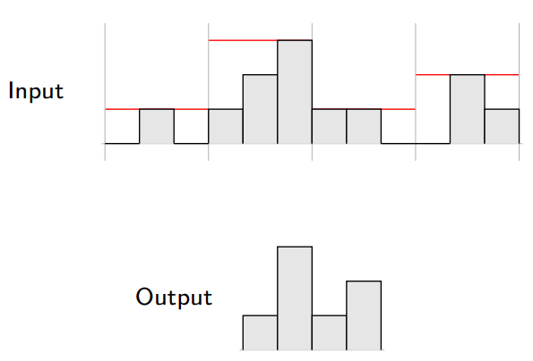
Pooling
When the input volume is large, pooling layers can be used to reduce the input dimension while preserving its global structure, in a way similar to a down-scaling operation.
Pooling
Consider a pooling area of size \(h \times w\) and a 3D input tensor \(\mathbf{x} \in \mathbb{R}^{C\times(rh)\times(sw)}\).
Max-pooling produces a tensor \(\mathbf{o} \in \mathbb{R}^{C \times r \times s}\) such that \[\mathbf{o}_{c,j,i} = \max_{n < h, m < w} \mathbf{x}_{c,rj+n,si+m}.\]
Average pooling produces a tensor \(\mathbf{o} \in \mathbb{R}^{C \times r \times s}\) such that \[\mathbf{o}_{c,j,i} = \frac{1}{hw} \sum_{n=0}^{h-1} \sum_{m=0}^{w-1} \mathbf{x}_{c,rj+n,si+m}.\]
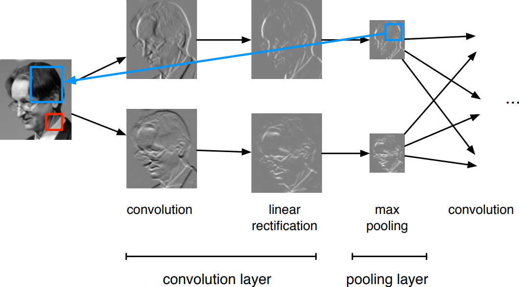
A convolutional network is generically defined as a composition of convolutional layers (\(\texttt{CONV}\)), pooling layers (\(\texttt{POOL}\)), linear rectifiers (\(\texttt{RELU}\)) and fully connected layers (\(\texttt{FC}\)).
The most common convolutional network architecture follows the pattern:
Note that for the last architecture, two \(\texttt{CONV}\) layers are stacked before every \(\texttt{POOL}\) layer. This is generally a good idea for larger and deeper networks, because multiple stacked \(\texttt{CONV}\) layers can develop more complex features of the input volume before the destructive pooling operation.
LeNet-5 (LeCun et al, 1998)
Composition of two \(\texttt{CONV}+\texttt{POOL}\) layers, followed by a block of fully-connected layers.
Composition of 5 VGG blocks consisting of \(\texttt{CONV}+\texttt{POOL}\) layers, followed by a block of fully connected layers. The network depth increased up to 19 layers, while the kernel sizes reduced to 3.
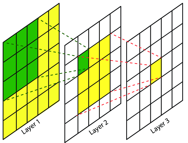
The effective receptive field is the part of the visual input that affects a given unit indirectly through previous convolutional layers. It grows linearly with depth.
E.g., a stack of two \(3 \times 3\) kernels of stride \(1\) has the same effective receptive field as a single \(5 \times 5\) kernel, but fewer parameters.
Composition of first layers similar to GoogLeNet, a stack of 4 residual blocks, and a global average pooling layer. Extensions consider more residual blocks, up to a total of 152 layers (ResNet-152).
Regular ResNet block vs. ResNet block with \(1\times 1\) convolution.
Training networks of this depth is made possible because of the skip connections in the residual blocks. They allow the gradients to shortcut the layers and pass through without vanishing.
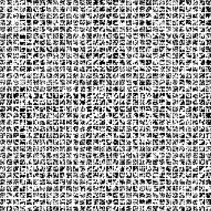
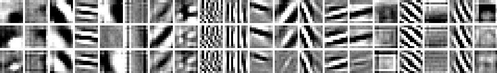
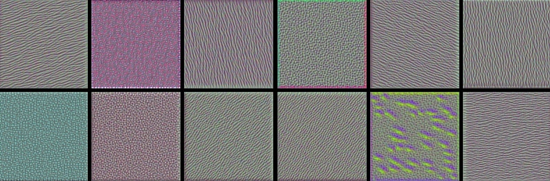
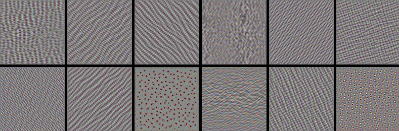
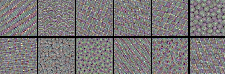
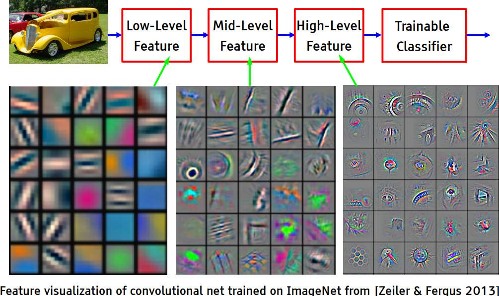
Convolutional networks can be inspected by looking for synthetic input images \(\mathbf{x}\) that maximize the activation \(\mathbf{h}_{\ell,d}(\mathbf{x})\) of a chosen convolutional kernel \(\mathbf{u}\) at layer \(\ell\) and index \(d\) in the layer filter bank.
These samples can be found by gradient ascent on the input space: \[\begin{aligned}
\mathcal{L}_{\ell,d}(\mathbf{x}) &= ||\mathbf{h}_{\ell,d}(\mathbf{x})||_2\\
\mathbf{x}_0 &\sim U[0,1]^{C \times H \times W } \\
\mathbf{x}_{t+1} &= \mathbf{x}_t + \gamma \nabla_{\mathbf{x}} \mathcal{L}_{\ell,d}(\mathbf{x}_t)
\end{aligned}\]
VGG-16, convolutional layer 1-1, a few of the 64 filters
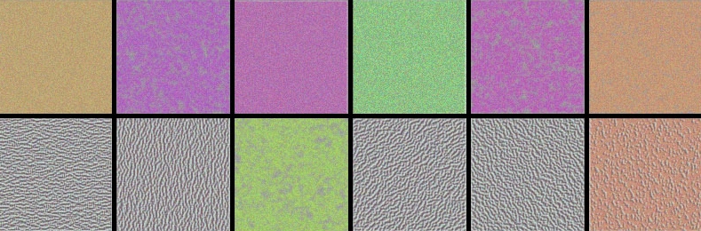
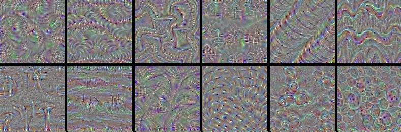
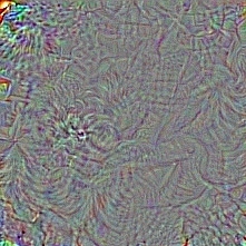
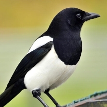
Deep Dream. Start from an image \(\mathbf{x}_t\), offset by a random jitter, enhance some layer activation at multiple scales, zoom in, repeat on the produced image \(\mathbf{x}_{t+1}\).
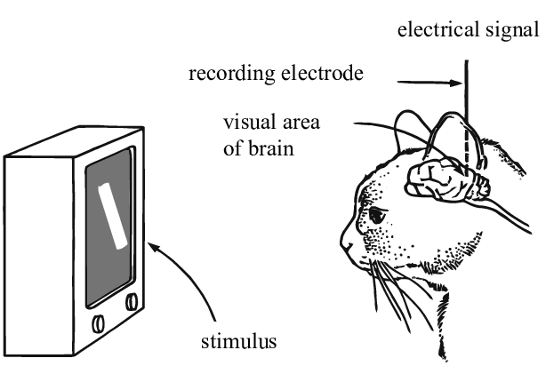
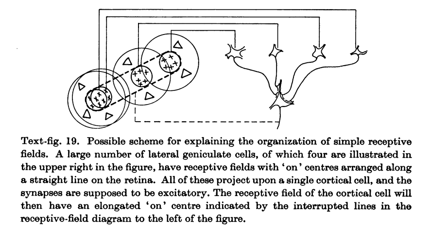
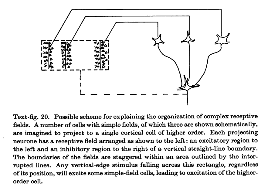
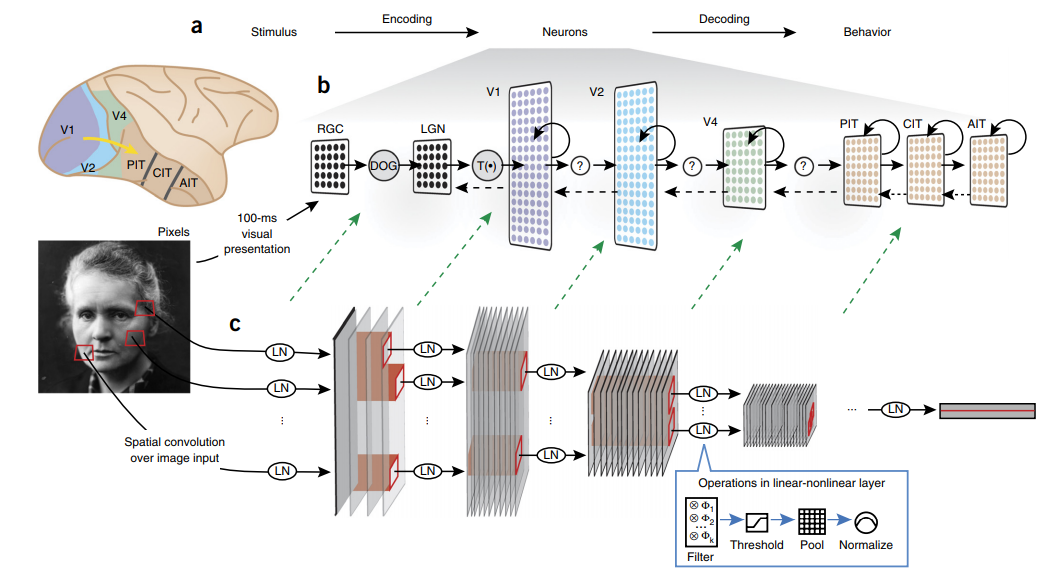
Biological plausibility
“Deep hierarchical neural networks are beginning to transform neuroscientists’ ability to produce quantitatively accurate computational models of the sensory systems, especially in higher cortical areas where neural response properties had previously been enigmatic.”
Credits: Yamins et al, Using goal-driven deep learning models to understand sensory cortex, 2016.