Machine Learning for Physics and Astronomy
Christoph Weniger
Tuesday, 7 Mar 2022
Chapter 4: Neural simulator-based inference
\(\newcommand{\indep}{\perp\!\!\!\perp}\)
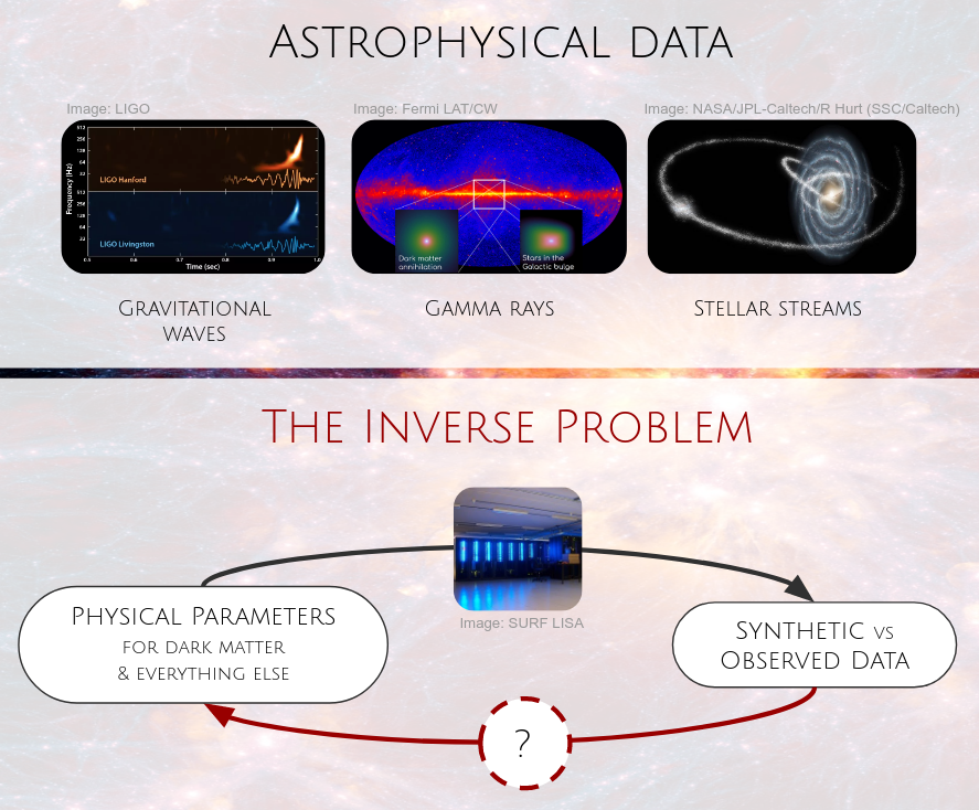
Recap - The inverse problem
![]()
Recap - Bayes theorem
Probabilistic inference using Bayes’ theorem
\[
P(Z|X) = \frac{P(X|Z)P(Z)}{P(X)}
\]
- \(P(X|Z)\): Probability of observation \(X\) given hypothesis \(Z\)
- \(P(Z)\): Our prior estimate of the truth of hypothesis \(Z\)
- \(P(Z|X)\): Probability of hypothesis \(Z\) given observation \(X\)
- \(P(X)\): Evidence. Probability of data \(X\) marginalized over all hypotheses \(Z\).
Likelihood-based inference is hard
Multimodal posteriors
![]()
In the case of multi-modal posteriors, MCMC methods like Metropolis-Hastings can get stuck in one of the modes instead of exploring all of them.
Image credit: Dynesty 1.1
Curse of dimensionality
![]()
In high dimensions, by far most of the volume of any region sits at the boundaries. This makes it increasingly hard to sample from the entire parameter space.
Image credit: Bishop 2007
No simulation reuse
![]()
Sometimes calculating the likelihood \(p(\mathbf x|z)\) of a specific parameter point \(z\) can be computationally very expensive. We cannot easily reuse these simulations in later runs.
Is there a smarter way of doing that with neural networks?
Neural simulator-based inference
Main idea: Instead of sampling from the posterior, we try to approximate it. There is quite a variety of techniques.
- “Posterior estimation”: estimate \(p(z|\mathbf{x})\) with a neural network.
- “Ratio estimation”: estimate \(p(\mathbf{x}|z)/p(\mathbf{x})\) with a neural network.
- “Likelihood estimation”: estimate \(p(\mathbf{x}|z)\) with a neural network.
This all falls broadly into the class of variational Bayesian methods. In this lecture we will discuss posterior and ratio estimation.
Posterior estimation
Let’s find some fitting function \(Q(z)\), aka variational posterior, such that \(Q(z) \approx P(z|x)\)
![]()
See Carleo, Giuseppe et al., 2019. “Machine Learning and the Physical Sciences.” http://arxiv.org/abs/1903.10563; Excellent overview: Zhang, Cheng et al. 2017. “Advances in Variational Inference.” http://arxiv.org/abs/1711.05597; also Cranmer, Kyle, Johann Brehmer, and Gilles Louppe. 2019. “The Frontier of Simulation-Based Inference.” http://arxiv.org/abs/1911.01429; Cranmer, Kyle, Juan Pavez, and Gilles Louppe. 2015. “Approximating Likelihood Ratios with Calibrated Discriminative Classifiers.” http://arxiv.org/abs/1506.02169
How to measure differences between probability distribution functions?
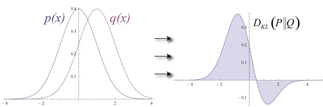
Posterior estimation with KL divergence
\[
D_{\rm KL}(P||Q) = \int p(x) \ln \left(\frac{p(x)}{q(x)}\right)dx
\]
Measures difference between probability density distributions.
![]()
- \(D_{\rm KL}(P||Q) = 0\) \(\Leftrightarrow\) \(p(x) = q(x)\)
- \(D_{\rm KL}(P||Q) \geq 0\)
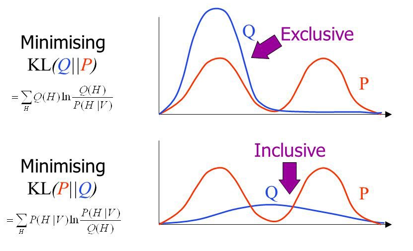
Failure modes of the KL divergence
What happens when approximating, say, a bi-modal function with a single mode?
Reverse KL divergence
- “mode seeking”
- good when aim is good fit to data
Forward KL divergence
- “mass covering”
- good when aim is conservative parameter constraints
Image credit: John Winn.
Forward KL divergence
Goal: Find \(q_\phi(z|x_0)\) for some observation \(x_0\) by minimize the KL divergence at \(x=x_0\)
\[
D_{\rm KL}(p||q) = \int p(z|x) \ln \left(\frac{p(z|x)}{q_\phi(z|x)}\right) dz
= \mathbb{E}_{z \sim p(z|x)} \left[\ln\frac{p(z|x)}{q_\phi(z|x)}\right]
\]
Approach: average over all possible observations, \(x\), and minimize
\[
\mathbb{E}_{x\sim p(x)}\left[ D_{KL}(p||q) \right] =
-\mathbb{E}_{x, z \sim p(x, z)} \ln q_\phi(z|x) + \text{const}
\]
This is simple: use gradient estimator
\[
\hat g_\phi(x) = - \nabla_\phi \ln q_\phi(z|x) \quad \text{with} \quad x, z\sim p(x, z)
\]
Result:
- an inference network \(q_\phi(z|x)\), that knows the posterior for all observations \(x\).
- just plug in \(x_0\), and \(q_\phi(z|x_0)\) is the answer.
- if you omit some \(z\), it learns the marginal posterior
Modeling posterior densities
Density estimation of \(q_\phi(z|x)\)
Pick parametric model \(q(z|\xi)\), and train NN to predict parameters \(\xi \equiv NN_\phi(x)\).
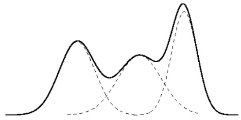
Gaussian mixture model
![]()
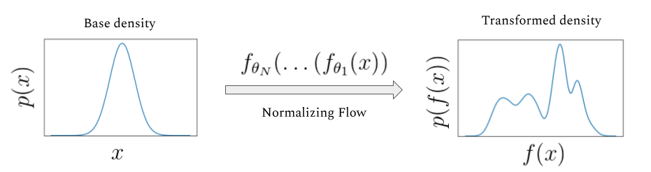
Normalizing flows
![]()
Image credit: https://siboehm.com/articles/19/normalizing-flow-network
Ratio estimation
Our goal is to approximate the “ratio” \[
r(\mathbf{x}, z)
\equiv \frac{p(\mathbf{x}, z)}{p(\mathbf{x})p(z)} = \frac{p(\mathbf x|z)}{p(\mathbf x)} = \frac{p(z|\mathbf x)}{p(z)}
\] This specific combination of probability densities is also known as point-wise mutual information. All equalities hold trivially due to various definitions of conditional probability distributions (see Bayes theorem).
Importantly: Since we know the prior \(p(z)\), learning this ratio is enough to estimate the posterior.
This requires loss functions that are different from forward KL. Connections between ratio and density estimation were e.g. discussed in Durkan, Conor et al. 2020. “On Contrastive Learning for Likelihood-Free Inference.” http://arxiv.org/abs/2002.03712
Neural likelihood-free inference
The surprising thing is that it is possile to estimate this ratio based on a simple binary classification task.
Goal: for any pair of observation \(\mathbf x\) and model parameter \(z\), the goal is to estimate the probability that this pair belongs one of the following classes
- \(H_0\): \(\mathbf x, z \sim P(\mathbf x, z)\)
- Data \(\mathbf x\) corresponds to model parameters \(z\).
- In practice, one could first draw \(z\sim p(z)\) from the prior, and then draw \(p(\mathbf x|z)\) from some simulator.
- \(H_1\): \(\mathbf x, z \sim P(\mathbf x)P(z)\)
- Data \(\mathbf x\) and model parameter \(z\) are unrelated and both independently drawn from their distributions.
See e.g. Louppe+Hermanns 2019 and references therein
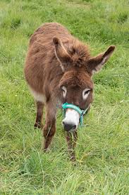
Joint vs marginal samples
- Examples for \(H_0\), jointly sampled from \(\mathbf x, z \sim P(\mathbf x|z) P(z)\)
Cat
![]()
Donkey
![]()
Cat
![]()
Cat
![]()
Donkey
![]()
Donkey
![]()
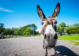
- Examples for \(H_1\), marginally sampled from \(\mathbf x, z \sim P(\mathbf x) P(z)\)
Donkey
![]()
Cat
![]()
Cat
![]()
Donkey
![]()
Cat
![]()
Donkey
![]()
Data: \(\mathbf x = \text{Image}\); Label: \(z \in \{\text{Cat}, \text{Donkey}\}\)
See Louppe+Hermanns 2019
Quiz
What loss function should one use?
Loss function
Strategy: We train a neural network \(d_\phi(\mathbf x, z) \in [0, 1]\) as binary classifier to estimate the probability of hypothesis \(H_0\) or \(H_1\). The network output can be interpreted, for a given input pair \(\mathbf x\) and \(z\), as probability that \(H_0\) is true.
- H0 is true: \(d_\phi(\mathbf x, z) \simeq 1\)
- H1 is true: \(d_\phi(\mathbf x, z) \simeq 0\)
The corresponding loss function is the binary cross-entroy loss
\[
L\left[d(\mathbf x, z)\right] = -\int dx dz \left[ p(\mathbf x, z) \ln\left(d(\mathbf x, z)\right) + p(\mathbf x)p(z) \ln\left(1-d(\mathbf x, z)\right) \right]
\]
Minimizing that function (see next slide) w.r.t. the network parameters \(\phi\) yields \[
d(\mathbf x, z) \approx \frac{p(\mathbf x, z)}{p(\mathbf x, z) + p(\mathbf x)p(z)}
\]
See Louppe+Hermanns 2019
Analytical minimization
We can formally take the derivative of the loss function w.r.t. network weights.
\[
\frac{\partial}{\partial\phi}
L \left[d_\phi(\mathbf x, z)\right] =
- \frac{\partial}{\partial\phi}
\int dx dz \left[ p(\mathbf x, z) \ln\left(d(\mathbf x, z)\right) + p(\mathbf x)p(z) \ln\left(1-d(\mathbf x, z) \right) \right]
\] \[
= -\int dx dz \left[ \frac{p(\mathbf x, z)}{d(\mathbf x, z)} - \frac{p(\mathbf x)p(z)}{1-d(\mathbf x, z) } \right] \frac{\partial d(\mathbf x, z)}{\partial \phi}
\]
Setting the part in square brackets to zero yields \[
d(\mathbf x, z) \simeq \frac{p(\mathbf x, z)}{p(\mathbf x, z) + p(\mathbf x)p(z)}\;,
\] which directly gives us our ratio estimator via \[
r(\mathbf x, z) \equiv \frac{d(\mathbf x, z)}{1- d(\mathbf x, z)} \simeq
\frac{p(\mathbf x|z)}{p(\mathbf x)}
= \frac{p(z|\mathbf x)}{p(z)} \;.
\]
How to do this in practice?
- Generate samples \(\mathbf x, z \sim p(\mathbf x|z) p(z)\) as training data.
- Define some network \(d_\phi(\mathbf x, z)\), which outputs values between zero and one (using sigmoid activation as last step).
- Optimize \(\phi\) using stochastic gradient descent.
Our above binary cross-entropy loss function can be equivalently written as \[
L\left[d(\mathbf x, z)\right] = -
\mathbb{E}_{
z\sim p(z), \mathbf x\sim p(\mathbf x|z), z'\sim p(z')}
\left[ \ln\left(d(\mathbf x, z)\right) + \ln\left(1-d(\mathbf x, z')\right) \right]\;.
\]
Estimates of this expectation value can be implemented in the training loop by first drawn pairs \(\mathbf x, z\) jointly and then drawing another \(z'\) from the prior.
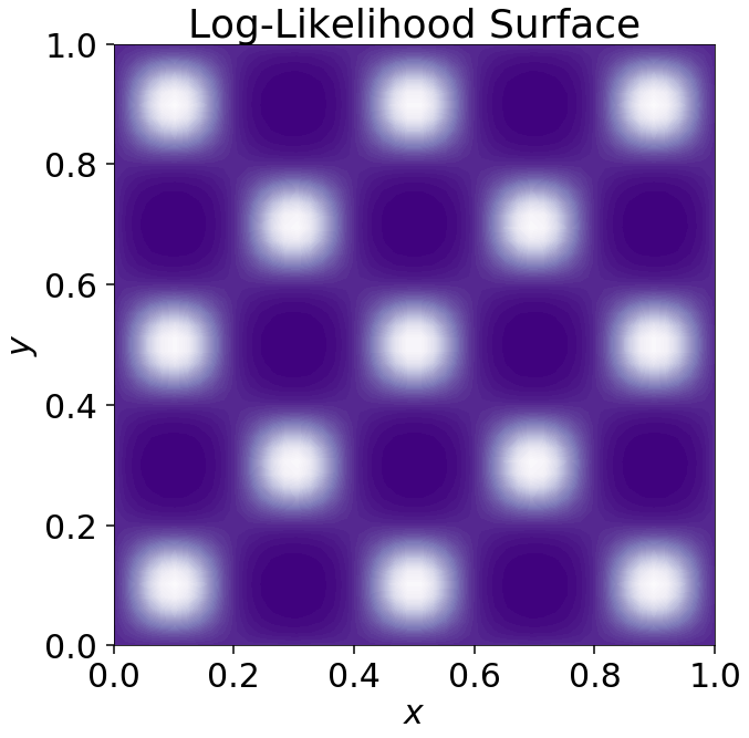
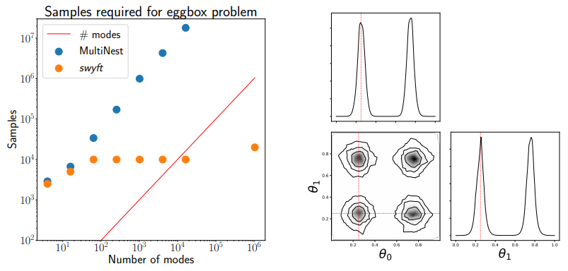
This method can give inference super powers
- Consider a high-dimensional eggbox posterior, with two modes in each direction. Assuming 20 parameters, this give \(2^{20} \sim 10^6\) modes.
- We can effectively marginalize over likelihoods with 1 Mio modes, using only 10 thousand samples.
![]()
From Miller+2020.
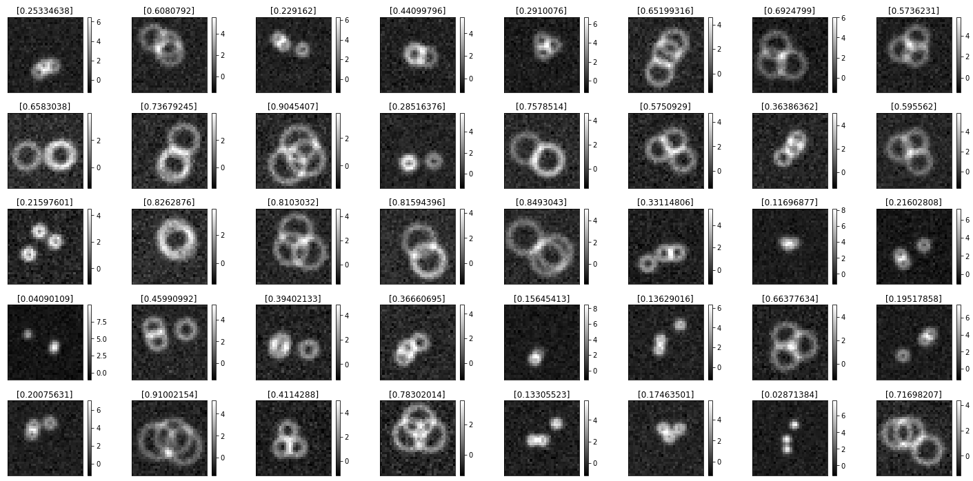
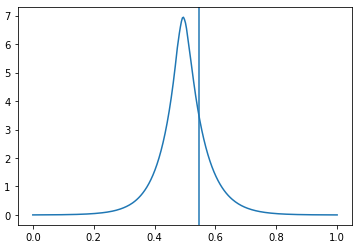
Exercises
shorturl.at/jmxL7
Your task: Estimate the radius, \(r \in [0, 1]\), of three rings, with a posterior.