Machine Learning for Astroparticle Physics:
A Crash-course in SBI

Lecture 4a: Normalising flows and other generative models

Christoph Weniger, University of Amsterdam (GRAPPA)

Normalising flows

A flexible density from invertible maps, via the change-of-variables formula.

Why we need flows

Real posteriors in physics are often multimodal, curved, or heavy-tailed. Gaussians can't represent them.

① Evaluate $\log q_\phi(\boldsymbol\theta\mid\mathbf{x})$

Needed for the NPE loss.

② Sample $\boldsymbol\theta \sim q_\phi$

Needed for corner plots, downstream analyses.

③ Arbitrary shape

Multimodal, curved, heavy-tailed.

MLPs on raw outputs fail ①: nothing forces normalisation.
Normalising flows satisfy all three by construction, via the change-of-variables formula.

The big picture

A simple base density $\pi_0(\mathbf{z}_0)$ is pushed through a chain of invertible maps $f_i$ into a complex target $\pi_K(\mathbf{z}_K)$.

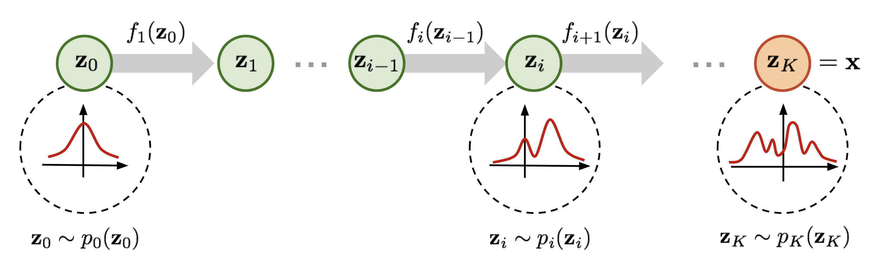
Figure: Lilian Weng, “Flow-based Deep Generative Models” (2018), lilianweng.github.io, after Weng's adaptation of Rezende & Mohamed (2015), arXiv:1505.05770.

Change of variables

Normalising flows are based on the change-of-variables formula.

Univariate case. If $z \sim p_Z(z)$ and $\theta = f(z)$ with $f$ invertible and differentiable, \[ p_\Theta(\theta) \;=\; p_Z(z)\,\left|\frac{dz}{d\theta}\right| \;=\; p_Z(f^{-1}(\theta))\,\left|\frac{df}{dz}\right|^{-1} \]

Multivariate case. For $\mathbf{z} \in \mathbb{R}^d$, and a mapping $\boldsymbol\theta = f(\mathbf{z})$, \[ p_\Theta(\boldsymbol\theta) \;=\; p_Z(f^{-1}(\boldsymbol\theta))\;\left|\det \frac{\partial f}{\partial \mathbf{z}}\right|^{-1} \] The Jacobian determinant is the volume rescaling. General $|\det J|$ costs $\mathcal{O}(d^3)$.

Example: warping a Gaussian

The volume compression can be nicely visualised in the univariate case.

map $\theta = z + A\sin z$

base $\mathcal{N}(0, 1.5^2)$

warped $p_\Theta(\theta) = p_Z(z)/|1+A\cos z|$

parameter $A$ = 0.80 monotonic ✓

Base $\mathcal{N}(0,1.5^2)$ pushed through $\theta = z + A\sin z$. For $A < 1$ the map is strictly monotonic, still invertible, but as $A\to 1$ the derivative near $z=\pm\pi$ collapses, so density mass piles up there: the warped target becomes bimodal.

Normalising flow = stack of invertible maps

to build a normalising flow, we now stack many simple invertible maps to generate a complex one.

\[ \boldsymbol\theta \;=\; f_L \circ f_{L-1} \circ \cdots \circ f_1(\mathbf{z}), \qquad \mathbf{z} \sim \mathcal{N}(0, I_d) \] Each $f_\ell$ is invertible and differentiable, with parameters $\phi_\ell$ (possibly conditioned on $\mathbf{x}$).

Sampling $\boldsymbol\theta \sim q_\phi$: draw $\mathbf{z}$, push forward through the stack.
Density evaluation at a given $\boldsymbol\theta$: invert the stack, evaluate $p_Z$, correct with Jacobians.
Composition of invertible maps is invertible, deep flows stay a valid density.

Flexibility grows with depth $L$, just like MLPs, but every layer preserves the probability axioms.

Log-density by chain of Jacobians

Evaluating the loss function (NLL) is formally straightforward.

Let $\mathbf{z}_\ell = f_\ell(\mathbf{z}_{\ell-1})$, $\mathbf{z}_0 = \mathbf{z}$, $\mathbf{z}_L = \boldsymbol\theta$. Change-of-variables composes: \[ \log q_\phi(\boldsymbol\theta\mid\mathbf{x}) \;=\; \log p_Z(\mathbf{z}_0) \;-\; \sum_{\ell=1}^{L} \log \left| \det \frac{\partial f_\ell}{\partial \mathbf{z}_{\ell-1}} \right| \]

Training is just minibatch SGD: \[ \mathcal{L}_{\mathrm{NPE}}(\phi) = -\frac{1}{|\mathcal{B}|}\sum_{(\boldsymbol\theta, \mathbf{x})\in\mathcal{B}} \log q_\phi(\boldsymbol\theta\mid\mathbf{x}) \]

Key design constraint: each $|\det \partial f_\ell / \partial \mathbf{z}_{\ell-1}|$ must be computationally cheap.

Example: Affine coupling layers

A specific type of mapping with cheap log determinant are affine coupling layers.

Idea: For each mapping, split parameters vector in two components $\mathbf{z} = (\mathbf{z}_A, \mathbf{z}_B)$. Define the transformation as \[ \mathbf{z}'_A = \mathbf{z}_A, \qquad \mathbf{z}'_B = \mathbf{z}_B \odot \exp\!\big(s_\phi(\mathbf{z}_A)\big) \;+\; t_\phi(\mathbf{z}_A) \] where $s_\phi, t_\phi$ are arbitrary neural networks (MLPs).

Invertibility
$\mathbf{z}_A$ passes through untouched; $\mathbf{z}_B$ is scaled-and-shifted given $\mathbf{z}_A$. Trivially invertible in closed form.

Cheap Jacobian
$J$ is triangular ⇒ $\log|\det J| = \sum_i s_\phi(\mathbf{z}_A)_i$. $\mathcal{O}(d)$, not $\mathcal{O}(d^3)$.

Then alternate which half is "active" across layer. Stack $L$ of these → expressive flow.

This is RealNVP: Dinh, Sohl-Dickstein & Bengio, “Density estimation using Real NVP” (2016), arXiv:1605.08803.

Why the Jacobian is cheap

Cheap Jacobian. $J$ is triangular ⇒ $\log|\det J| = \sum_i s_\phi(\mathbf{z}_A)_i$, so the cost is $\mathcal{O}(d)$, not $\mathcal{O}(d^3)$.

Flow pushforward, live 2D demo

Base $z\sim\mathcal{N}(0,I)$

→

after $f_1$

→

after $f_2$

→

after $f_3$

→

Data $x=f_\theta(z)$

Flow: 4 affine coupling layers, MLP(32). Target: banana (grey). Loss: $-\mathbb{E}[\log q_\theta(x)]$

      step: 0   loss: —
    

Colours tag fixed $z$-points by angle, watch each coupling layer bend the cloud step by step into the banana.

Trained live in your browser with TF.js. Each layer: $x_b = z_b \cdot e^{s(z_a)} + t(z_a)$, swapping $a\leftrightarrow b$. Exact log-density via $\log|\det J| = \sum_\ell s_\ell$.

Conditional flows, plugging in the data

From modeling densities to modeling conditional densities.

For SBI we want $q_\phi(\boldsymbol\theta \mid \mathbf{x})$, not just $q_\phi(\boldsymbol\theta)$. To that end, the scale and shift networks should be data dependent (potentially through an embedding $T_\phi(\mathbf{x})$): \[ s_\phi(\mathbf{z}_A) \to s_\phi(\mathbf{z}_A, T_\phi(\mathbf{x})), \qquad t_\phi(\mathbf{z}_A) \to t_\phi(\mathbf{z}_A, T_\phi(\mathbf{x})) \]

Full picture

Embedding $T_\phi(\mathbf{x})$ compresses the data (CNN / Transformer / GNN, see Lec 4).
Conditional flow turns $\mathbf{z}\sim\mathcal{N}(0,I)$ into $\boldsymbol\theta$, with all coupling-layer parameters depending on $T_\phi(\mathbf{x})$.
Loss: $-\log q_\phi(\boldsymbol\theta^\star\mid\mathbf{x})$ averaged over simulator pairs.

Every component, embedding and coupling networks $s, t$, is trained together by backprop.

Other generative models, at a glance

Coupling normalising flows are but one choice of conditional head $q_\phi(\boldsymbol\theta\mid\mathbf{x})$. Others trade exact density for scale or speed:

Discrete normalising flows (RealNVP, neural spline, ...). Low to moderate dim ($\lesssim 100$), exact density, fast sampling.
Continuous normalising flows (neural ordinary differential equation, ODE). Normalising flow with "infinite steps"; exact density via ODE; training/sampling requires ODE.
Flow matching. Similar to continuous normalising flows, but without ODE solve during training (much faster).
Diffusion / score-based (neural stochastic differential equation, SDE). For high-dimensional, image- or field-shaped data; fast training; slow sampling (requires SDE).
Autoregressive models / Transformers Can handle varying parameter dimensionality (transdimensional), exact likelihoods, but sampling is sequential and can be slow.
Cross entropy/classification. Discrete parameters, closed-form conditional, simple and fast.

Example: stochastic GW background with LISA

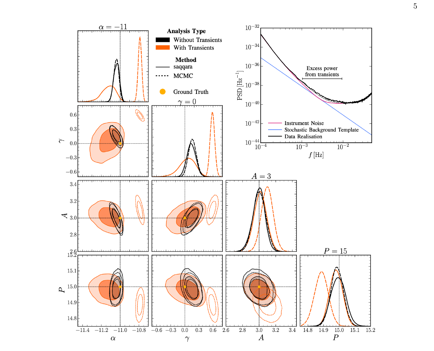
Here the parameter $\boldsymbol\theta$ is four-dimensional, and describes properties of the stochastic GW background and noise model. We estimate the posterior $q_\phi(\boldsymbol\theta\mid\mathbf{x})$ based on synthetic LISA data.

Normalising flows allow to model non-Gaussian (here potato-shaped) posteriors, which are common in physics.

Example: reconstruction of the initial matter density field

Here the parameter describes the initial density field at redshift $z=1000$, and it is $64\times64\times64 = 262144$ dimensional. We estimate the posterior $q_\phi(\boldsymbol\theta\mid\mathbf{x})$ based todays density field.

The posterior is approximated as a multivariate Gaussian, $q_\phi(\boldsymbol\theta\mid\mathbf{x}) = \mathcal{N}(\boldsymbol\mu_\phi(\mathbf{x}), \Sigma_\phi(\mathbf{x}))$.

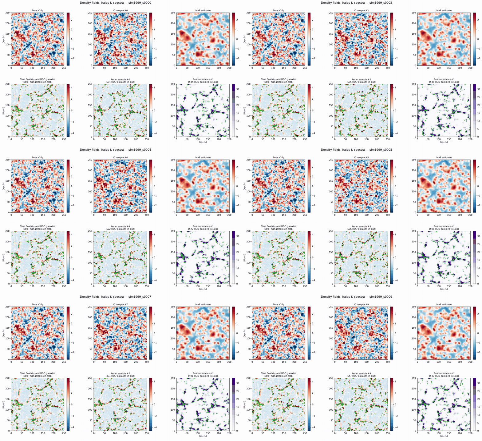(Preliminary, Oleg Savchenko, in preparation)

What next?

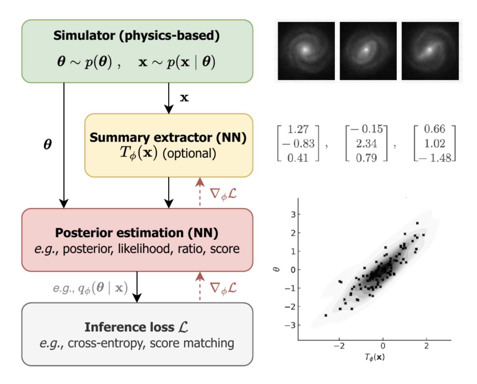
We now discussed the red block in the diagram below: the conditional head $q_\phi(\boldsymbol\theta\mid\mathbf{x})$ can be a normalising flow, or any other generative model. Next we will discuss a classical example for a summary network $T_\phi(\mathbf{x})$, the CNN.

Machine Learning for Astroparticle Physics: A Crash-course in SBI