Motivation > Open questions
Fundamental questions about the physics of the Universe
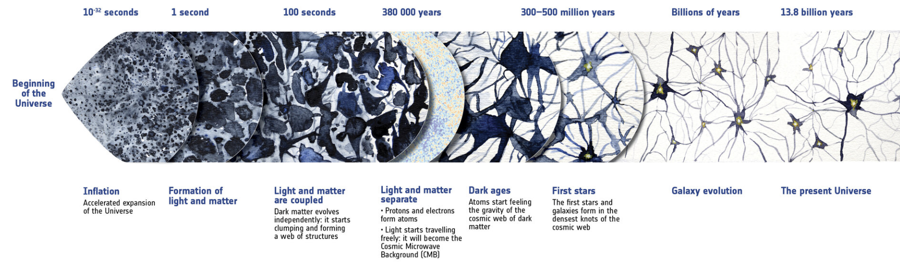
Questions guiding searches for new fundamental physics (from CERN, ESA, APPEC, ASTRONET roadmaps):
- What is the nature of dark matter and dark energy?
- What are the fundamental properties of neutrinos and their cosmic role?
- What can multi-messenger observations (\(\gamma\), \(\nu\), CRs, GWs) reveal about the extreme Universe?
- How did the first stars / galaxies / black holes form, and how does the Milky Way fit in?
- What more can we learn about the early Universe (CMB and related probes)?
- How can extreme objects and processes serve as laboratories for new fundamental physics?
Image credit: ESA
Motivation > The inverse problem
Forward simulation and the inverse problem
what we care about
BH masses, lens profile, ...
forward — physics knowledge and assumptions
inverse — generating insights
what we observe
power spectra, …
Note: SBI requires samples from \(p(\mathbf{x}\mid\boldsymbol\theta)\), i.e. running simulator, for comparison with \(\mathbf{x}_{\rm obs}\). Likelihood-based methods need pointwise evaluations of \(p(\mathbf{x}_{\rm obs}\mid\boldsymbol\theta)\), i.e. evaluating the likelihood function.
Motivation > A short history
Bayesian inference in practice
We always want the posterior \(p(\boldsymbol\theta\mid\mathbf{x})\); only its representation changes: formula → samples → network.
conjugate priors
optimisation
Motivation > Applications
Application so SBI
Neural SBI is run and stress-tested with full instrumental forward models across astroparticle physics and cosmology. Four examples:
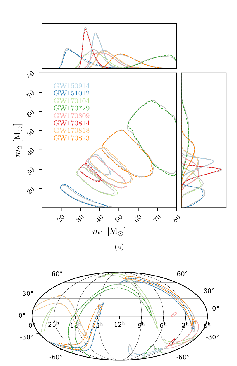
Dax et al. 2021, arXiv:2106.12594
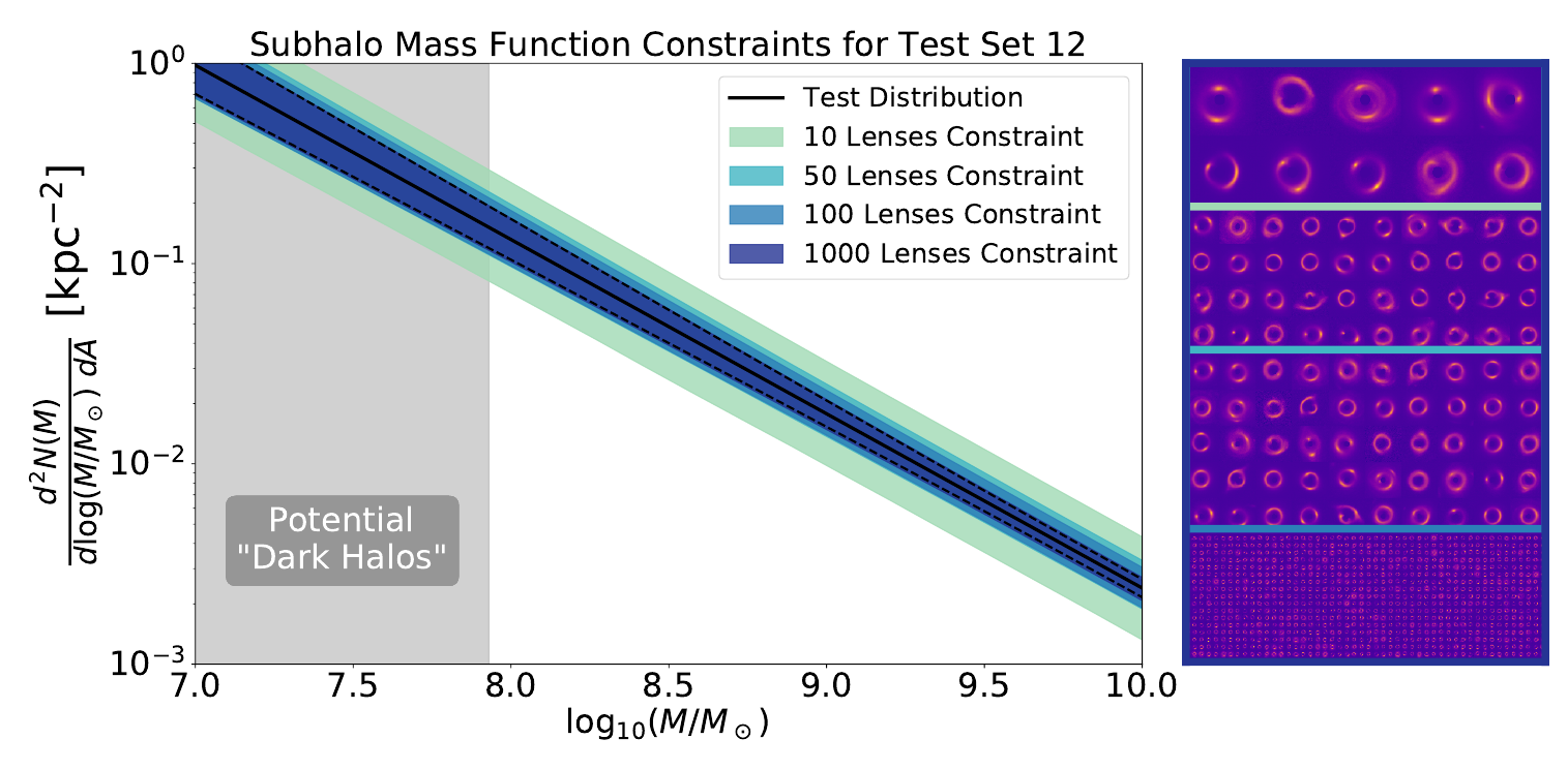
arXiv:2203.00690
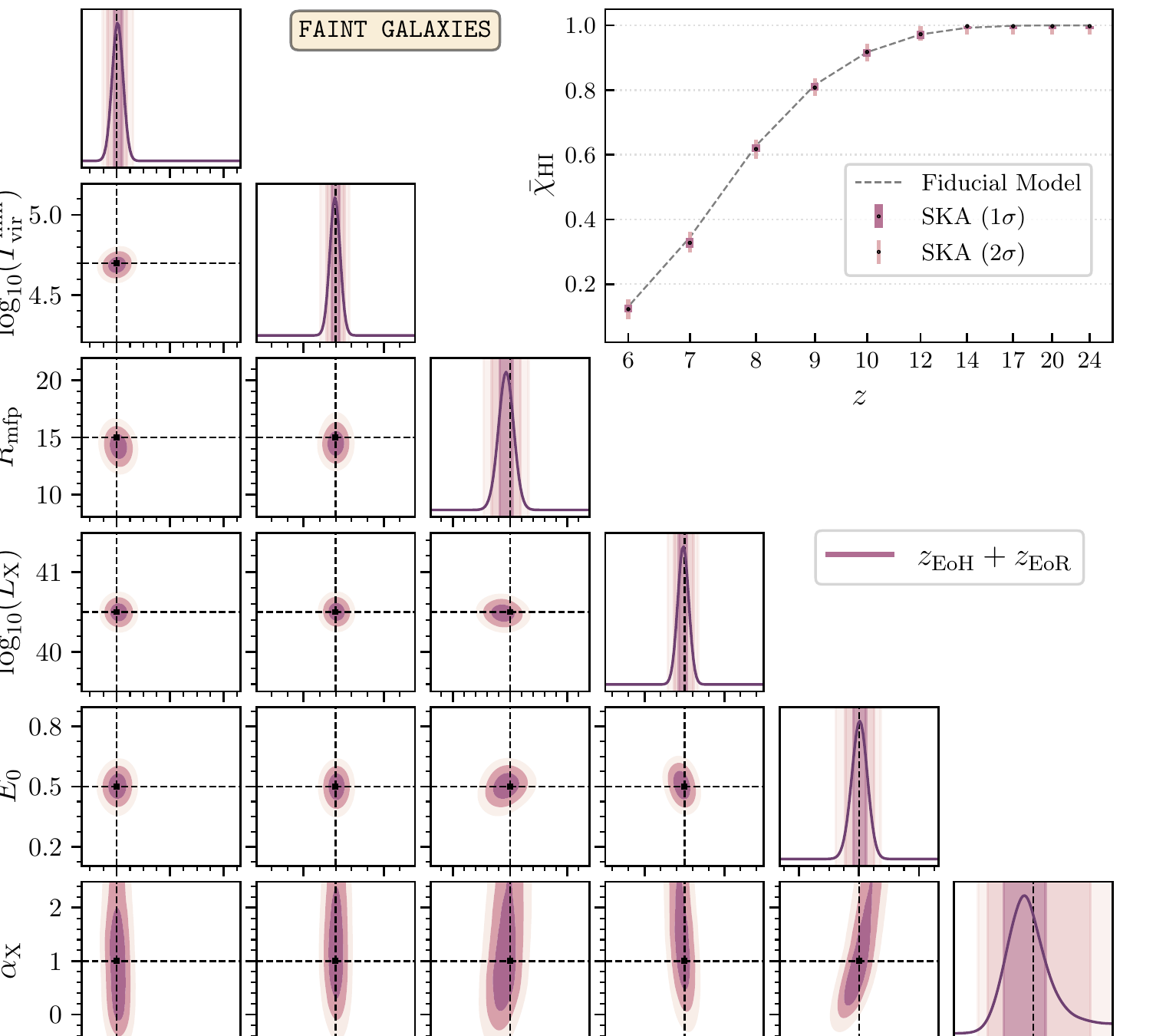
arXiv:2303.07339
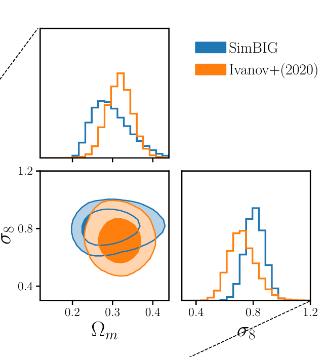
arXiv:2211.00723
Motivation > Simulation efficiency
Higher simulation efficiency
Increases simulation efficiency (LBI to SBI)
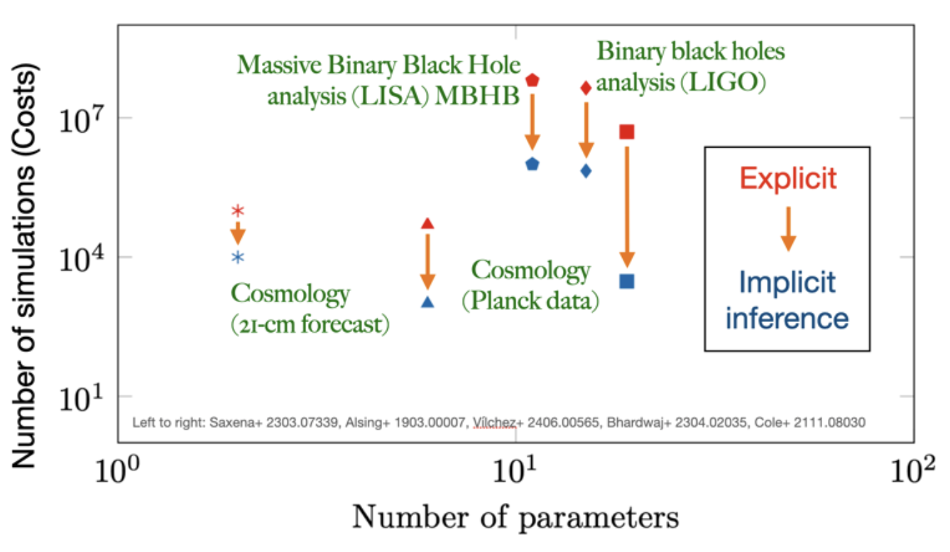
Figure credit: Noemi Anau Montel
Motivation > Plan
Plan for these two lectures
In this course we will introduce the foundational concepts of simulation-based inference. We will introduce key concepts step-by-step, with multiple examples to develop intuition. The hands-on exercises will support this.
- Approximate Bayesian computation
- The four components of neural SBI
- Density estimation and learned summaries
- Diagnostics and failure modes
- Sequential and dynamic SBI
- Towards complex analysis problems
Classical SBI > The forward model
Simulation-based inference
We model a ball, thrown at an angle \(\theta\) with initial speed \(v\), which hits the ground at an observed distance \(x\). The measurement noise is Gaussian.
\( \theta \sim \mathcal{U}(5^\circ,85^\circ),\ \ v \sim \mathcal{N}(10,0.2^2),\ \ x \sim \mathcal{N}\!\big(\tfrac{v^2}{g}\sin 2\theta,\ 0.5^2\big) \)
Each shot is one draw \((\theta, x)\) from the simulator — the cloud is the joint \(p(\theta, x)\).
Classical SBI > Simulator vs likelihood
Forward model — simulator vs likelihood
Depending on whether the likelihood \(p(x\mid\theta)\) is available explicitly or implicitly, different inference modes are available.
Explicit likelihood
Requires integration over \(v\).
Implicit likelihood (Simulator)
Classical SBI > Rejection ABC
Rejection ABC — From joined to posterior samples
Rank the simulations against \(x_\mathrm{obs}\), keep the closest, a histogram gives the posterior.
- \(M\) trades bias against noise. Too small and the peaks drown in Monte Carlo noise; too large and the histogram leaks back toward the prior.
- Sharper costs simulations. Shrinking \(\varepsilon_\mathrm{eff}\) at fixed \(M\) means throwing more \(N\) at it — the sample-efficiency cliff.
- But it is amortised. Moving \(x_\mathrm{obs}\) re-ranks the same cloud, for free.
Classical SBI > Kernel density estimation
Taking the tolerance to zero, done right
Interpolate in the joined \((\theta, x)\)-space instead of accepting and rejecting — the \(\varepsilon \to 0\) limit.
- Nothing is rejected. Every simulation contributes, weighted by \(w_i = K_{h_x}(x_\mathrm{obs}-x_i)\) — at the same \(N\) as rejection ABC the bimodal structure comes out cleanly.
- The bandwidth replaces the tolerance. \(h_x\) plays \(\varepsilon\)'s role but is chosen automatically; here \(h_x \approx \sigma\) is the right answer.
Beaumont, Zhang & Balding 2002, Genetics 162, 2025 (kernel-weighted ABC) · Blum 2010, JASA 105, 1178 · Silverman 1986 (KDE).
Classical SBI > Rejection ABC
Rejection ABC — the general components
Three steps. Every method in this lecture is a different choice at each one — rejection ABC makes the simplest choice available.Simulate
Draw \(\boldsymbol\theta\sim p(\boldsymbol\theta)\) and run the simulator forward to get \(x\).
Compress
Reduce the data to a summary \(s(x)\) low-dimensional enough to compare.
Construct posterior
Keep the \(\boldsymbol\theta\) whose summaries came out close to \(s(x_\mathrm{obs})\).
In the live demos \(\varepsilon\) is replaced by "keep the top-\(M\) closest of \(N\)".
Rubin 1984, Ann. Statist. 12, 1151 (the loop on paper) · Pritchard et al. 1999, Mol. Biol. Evol. 16, 1791 (the name "ABC") · Sisson, Fan & Beaumont 2018, Handbook of ABC.
Classical SBI > Takeaways
Key takeaways — rejection ABC
Generic properties and challenges with this approach.
Works generically (and keeps working)
- Amortised inference. Pay the simulation cost once; any new observation \(x_\mathrm{obs}\) is then a free query.
- No likelihood evaluations. Only simulator samples are needed, never a pointwise \(p(x\mid\theta)\) evaluation.
- Trivial marginalisation. Nuisances (here the muzzle speed \(v\)) fold in for free by sampling them inside the simulator.
Stays hard (what the rest of this lecture is about)
- Summary construction. We only had one observable, for higher dimensional data we need sufficient data summaries. Hand-picked summaries do not scale to images, waveforms or graphs.
- Density estimation in high D. Our demo was 1-dimensional; with many parameters histogram loses meaning and smoothing becomes hard.
Neural SBI > Overview
The four building blocks of an SBI analysis
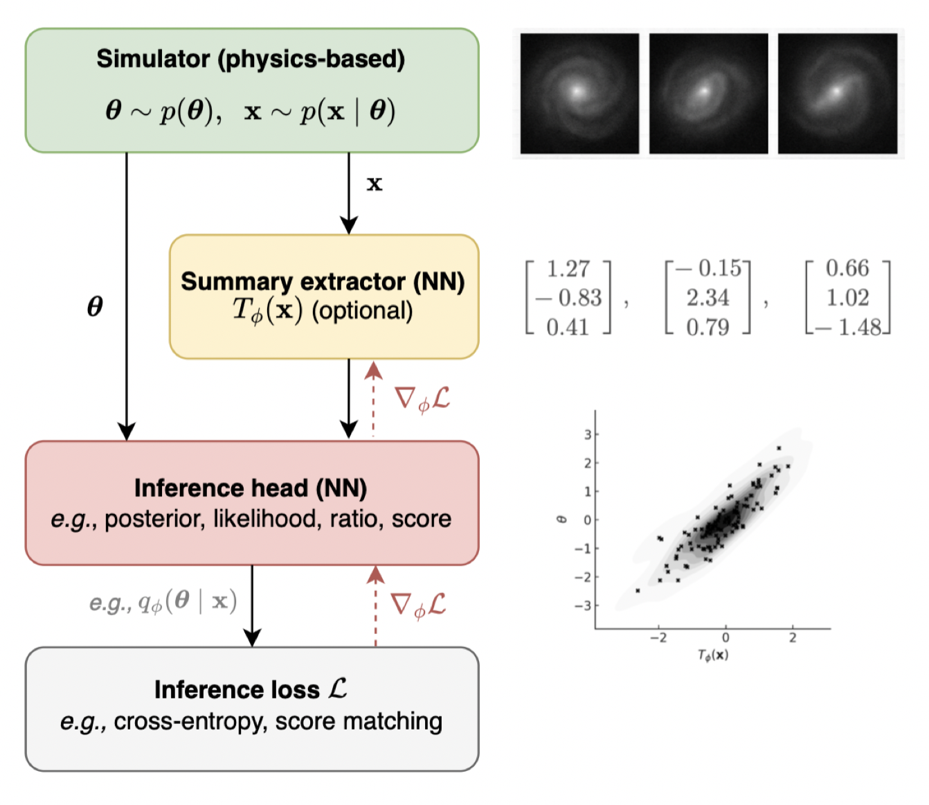
The simulator holds our knowledge about the considered system, and
emits nothing but pairs \((\boldsymbol\theta, \mathbf{x})\).
The summary extractor \(T_\phi(\mathbf{x})\) filters out the
relevant information for inference.
The inference head \(q_\phi\) learns the answer.
And the inference loss \(\mathcal{L}\) defines the question:
change it, and the inference head learns a posterior, a likelihood, a ratio, a score, ...
Both the summary extractor and the inference head are often trained end-to-end, by a single gradient \(\nabla_\phi \mathcal{L}\).
Neural SBI > I. Simulators
I. Simulators
Everything downstream inherits its assumptions.
Neural SBI > I. Simulators
Some example simulators
Simulators come in a wide range of runtimes and data shapes.
| Example | runtime / call | \(d_\theta\) | \(d_x\) | What makes it awkward |
|---|---|---|---|---|
| Cannon ball (this lecture) | μs | 1 | 1 | Nothing. That is the point of a toy. |
| CBC waveform + detector noise | 10 ms – 10 s | 11 – 17 | \(10^4\) – \(10^6\) | Non-stationary PSD, glitches, calibration. |
| Strong-lens image (galaxy + subhaloes) | 0.1 – 10 s | 10 – \(10^3\) | \(10^4\) – \(10^6\) | Transdimensional: the number of parameters is itself random. |
| N-body / hydro cosmological box | \(10^3\) – \(10^6\) h | 5 – 20 | \(10^6\) – \(10^9\) | Budget-bound: a few thousand runs, ever. |
| LISA global fit | minutes | \(10^4\) – \(10^5\) | \(10^7\)+ | Thousands of overlapping sources, count unknown. |
| IceCube event reconstruction | ms – s | 5 – 10 | \(10^3\) – \(10^5\) | A point cloud, not a grid. |
Neural SBI > II. Training targets
II. Training targets
The loss defines the question. Same simulator, same network, different answer: posterior, likelihood, or ratio.
Neural SBI > II. Training targets
Three questions you can ask of the same simulations
Neural SBI > II. Training targets · NPE
Neural posterior estimation
Simulate once from the prior, then fit a conditional density by maximum likelihood. That is the whole algorithm.
Step 1: generate training data
Step 2: train the density estimator
with \(q_\phi(\boldsymbol\theta\mid\mathbf{x}) \ge 0\) and \(\int d\boldsymbol\theta\, q_\phi(\boldsymbol\theta\mid\mathbf{x}) = 1\) — the two constraints the architecture must enforce.
Result: the posterior, amortised
Papamakarios & Murray 2016, arXiv:1605.06376 (NPE, with a mixture-density head) · Lueckmann et al. 2017, arXiv:1711.01861 · Greenberg et al. 2019, arXiv:1905.07488 · review: Cranmer, Brehmer & Louppe 2020, arXiv:1911.01429 (PNAS 117, 30055).
Neural SBI > II. Training targets · NPE
Mathematical justification
Take two idealisations: (i) Infinite training data, \(N\to\infty\). (ii) The network is infinitely flexible, so \(q(\boldsymbol\theta\mid\mathbf{x})\) is any non-negative, normalised function with \(\int q(\boldsymbol\theta\mid\mathbf{x})\,d\boldsymbol\theta = 1\).
\[ \mathcal{L}[q] \;\longrightarrow\; -\!\iint p(\boldsymbol\theta, \mathbf{x})\, \log q(\boldsymbol\theta\mid\mathbf{x})\, d\boldsymbol\theta\, d\mathbf{x} \]
\[ \mathcal{L}[q] = \mathbb{E}_{\mathbf{x}}\!\big[\mathrm{KL}\!\left(p(\cdot\mid\mathbf{x})\,\|\,q(\cdot\mid\mathbf{x})\right)\big] + H(\boldsymbol\theta\mid\mathbf{x}) \]
The entropy term does not depend on \(q\). KL \(\ge 0\) with equality iff \(q = p(\cdot\mid\mathbf{x})\), so
\[ q^\star(\boldsymbol\theta\mid\mathbf{x}) = p(\boldsymbol\theta\mid\mathbf{x}). \]
The learned \(q_\phi(\boldsymbol\theta\mid\mathbf{x})\) is the Bayesian posterior implied by the simulator. A finite network with finite training just interpolates this idealised answer.
Neural SBI > II. Training targets · NPE
The Gaussian-head network
The simplest ansatz for \(q_\phi\).
A simple Gaussian density model.
\( q_\phi(\boldsymbol\theta\mid x) \;=\; \mathcal{N}\!\bigl(\boldsymbol\theta\,\big|\,\boldsymbol\mu_\phi(x), \boldsymbol\Sigma_\phi\bigr) \)
Only the mean depends on \(x\); \(\boldsymbol\Sigma_\phi\) is a free parameter shared by every \(x\). A homoscedastic head learns how confident to be, just not where.
NPE loss on simulator pairs \((\boldsymbol\theta_n, x_n)\):
\( \mathcal{L}(\phi) = -\tfrac{1}{N}\sum_n \log q_\phi(\boldsymbol\theta_n\mid x_n) \)
For diagonal \(\Sigma\) this is \(\tfrac{1}{2}\bigl((\theta-\mu)/\sigma\bigr)^2 + \log\sigma\) per parameter. Freeze \(\Sigma\) and it reduces to mean-squared error.
// Train q_phi(theta|x) on simulator pairs (theta_n, x_n)
// log_sigma: free parameter, not a function of x
for step = 1, 2, ... :
    sample mini-batch B of pairs
    mu = f_phi(x)
    L = mean( 0.5*((theta-mu)/sigma)^2 + log_sigma )
    (phi, log_sigma) <- Adam(., grad L)
Neural SBI > II. Training targets · NPE
Live demo — Gaussian head on a linear forward model
Forward model: \(t_i = a + b\,x_i + \varepsilon\), 20-point grid, \(\varepsilon\sim\mathcal{N}(0,0.25^2)\). Priors \(a\sim\mathcal U[-1,1]\), \(b\sim\mathcal U[-2,2]\). Network: MLP \([20{\to}32{\to}16{\to}2]\), output \((\mu_a,\mu_b)\); \(\log\sigma_a,\log\sigma_b,\rho\) are three free trainable scalars, shared across all \(\mathbf{x}\).
Left: a single observation \(\mathbf{x}\). Right: the learned posterior \(q_\phi(a,b\mid\mathbf{x})\) (orange ellipse) against the true \((a^\star,b^\star)\) (green star). The same trained network handles any new \(\mathbf{x}\): amortised inference.
Applications > Native capabilities of SBI
Example: Inferring field configurations in cosmology
Inference of millions of parameters at once is possible, e.g. a full 3D field of initial conditions for cosmological structure formation.
- Target the full posterior \(q(\mathbf{z}\mid\mathbf{x})\) over an entire field (here \(64^3\) initial conditions), not just a handful of parameters.
- A U-Net encoder–decoder parametrises the map from data to field, scaling to millions of dimensions. \[\mu_\phi(\mathbf{x}) = \text{UNet}_\phi(\mathbf{x})\]
- Structural assumptions accelerate training: model \(q\) as a Gaussian with a specific (structured) covariance, e.g. learned in precision space. \[Q_L = D_2 \mathcal{H} D_1 \mathcal{H} D_2\]
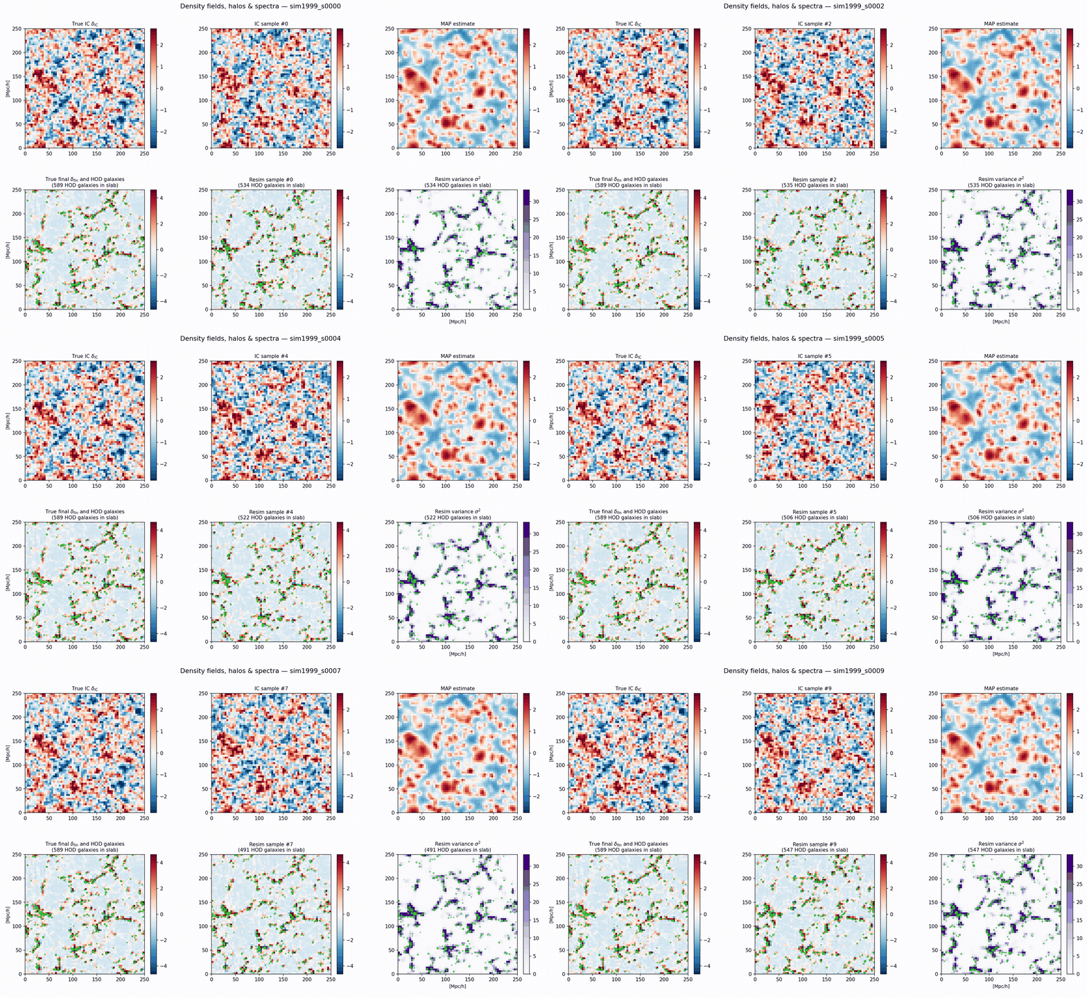
O. Savchenko et al., in prep. — Falcon + Disco-DJ
See also: Jasche & Wandelt 2013 (BORG), arXiv:1203.3639 · Doeser et al. 2024, arXiv:2312.09271
PRELIMINARY
Neural SBI > II. Training targets · NLE / NRE
Learning the likelihood, or just the ratio
Same simulator, similar network. Changing the loss changes the target.
Fit the conditional density in the other direction:
The minimiser is \(p(\mathbf{x}\mid\boldsymbol\theta)\): a surrogate likelihood for any sampler. Prior-free, but sampling costs an MCMC run.
Do not model a density. Train a classifier with binary cross entropy loss to tell joint pairs, \(x, \theta \sim p(x\mid \theta)p(\theta)\), from shuffled ones, \(x, \theta \sim p(x)p(\theta)\). Its optimum is
No normalisation constraint. Sampling again needs MCMC.
Cranmer, Pavez & Louppe 2015, arXiv:1506.02169 (the likelihood-ratio trick these rest on) · Papamakarios, Sterratt & Murray 2019, arXiv:1805.07226 (SNL) · Hermans, Begy & Louppe 2020, arXiv:1903.04057 (AALR) · Miller et al. 2021, arXiv:2107.01214 (TMNRE).
Neural SBI > II. Training targets
NPE, NRE, NLE
Comparison of the three main flavours of neural SBI. All three are trained on the same simulator pairs, but they answer different questions.| NPE | NRE | NLE | |
|---|---|---|---|
| Models | \(q_\phi(\boldsymbol\theta\mid\mathbf{x})\) | \(\log r_\phi(\boldsymbol\theta, \mathbf{x})\) | \(q_\phi(\mathbf{x}\mid\boldsymbol\theta)\) |
| Loss | Negative log likelihood (NLL) | cross-entropy | NLL |
| Sampling | direct, single forward pass | MCMC on \(p(\boldsymbol\theta)\,e^{f_\phi(\boldsymbol\theta, \mathbf{x})}\) | MCMC on \(q_\phi(\mathbf{x}\mid\boldsymbol\theta)\,p(\boldsymbol\theta)\) |
| Amortised | yes | yes (re-MCMC per obs) | partial (re-MCMC per obs) |
| Prior can change after training | no | yes | yes |
| High-D \(\boldsymbol\theta\) | Adopt any high-dim generative model | hard, scales via targeting marginals | hard, \(\mathbf{x}\) often higher-D |
| Data summaries | learned end-to-end | learned end-to-end | must be provided |
Neural SBI > III. Density estimation
III. Density estimation
The head has to be a probability density: non-negative, normalised, fast to evaluate and fast to sample.
Neural SBI > III. Density estimation
Representing a probability density is hard
We need to approximate probability distributions, \( q_\phi(\theta \mid x) \approx p(\theta \mid x) \), given only samples from a simulator. These are highly constrained objects.
What a density must satisfy
Non-negative, \(q_\phi(\theta)\ge 0\).
Easy, exponentiate.
Normalized, \(\int q_\phi(\theta)\,d\theta = 1\).
Hard. This is a global
constraint: change the network anywhere and the integral changes everywhere.
And two operations, both fast
Evaluate, given \(\theta\), return \(q_\phi(\theta)\).
Importance weights, likelihoods, model comparison.
Sample, draw fresh \(\theta \sim q_\phi\).
Error bars, corner plots, propagating uncertainty.
Both get called millions of times in a real analysis, so "fast" is part of the specification, not a nicety. No classical representation gives you all of this at once.
Neural SBI > III. Density estimation · Normalising flows
The big picture
A simple base density \(\pi_0(\mathbf{z}_0)\) is pushed through a chain of invertible maps \(f_i\) into a complex target \(\pi_K(\mathbf{z}_K)\).
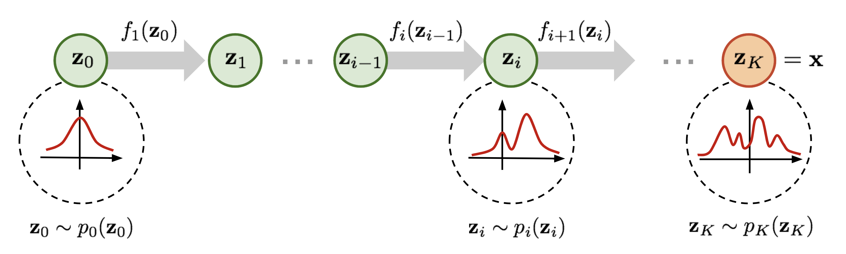
After Rezende & Mohamed (2015), arXiv:1505.05770.
Neural SBI > III. Density estimation · Normalising flows
Normalising flows in three equations
A normalising flow is cheap to sample and exact to evaluate. The learned object is the map itself: a chain of invertible layers \(f_\phi = f_L\circ\cdots\circ f_1\) taking Gaussian noise to \(\boldsymbol\theta\). For SBI it is conditional, \(q_\phi(\boldsymbol\theta\mid\mathbf{x})\), with \(\mathbf{x}\) fed to the networks inside each layer.1. Sample. Push a Gaussian draw through the chain — one forward pass, no integration:
2. Evaluate. Change of variables — exact, closed form, one backward pass:
3. Train. Maximum likelihood on that exact log-density — no regression surrogate, no trajectories to simulate:
Exact likelihood in one pass. The price: every layer invertible, every \(\det J\) cheap.
Rezende & Mohamed 2015, arXiv:1505.05770 · Dinh et al. 2016, arXiv:1605.08803 · Papamakarios et al. 2017, arXiv:1705.07057 · Papamakarios et al. 2021 (review), arXiv:1912.02762
Neural SBI > III. Density estimation · Normalising flows
Example: affine coupling layers
A specific type of mapping with cheap log determinant are affine coupling layers.\(\mathbf{z}_A\) passes through untouched; \(\mathbf{z}_B\) is scaled-and-shifted given \(\mathbf{z}_A\). Trivially invertible in closed form.
\(J\) is triangular ⇒ \(\log|\det J| = \sum_i s_\phi(\mathbf{z}_A)_i\). \(\mathcal{O}(d)\), not \(\mathcal{O}(d^3)\).
Then alternate which half is "active" across layer. Stack \(L\) of these → expressive flow.
This is RealNVP: Dinh, Sohl-Dickstein & Bengio 2016, “Density estimation using Real NVP”, arXiv:1605.08803.
Neural SBI > III. Density estimation · Normalising flows
Flow pushforward, live 2D demo
A normalising flow is a chain of invertible maps \(f_\ell\) that push a simple base density into a complex target. The demo below shows the intermediate distributions after each layer.Colours tag fixed \(z\)-points by angle. Watch each coupling layer bend the cloud step by step into the banana.
Trained live in your browser with TF.js. Each layer: \(x_b = z_b \cdot e^{s(z_a)} + t(z_a)\), swapping \(a\leftrightarrow b\). Exact log-density via \(\log|\det J| = \sum_\ell s_\ell\).
Neural SBI > III. Density estimation · Normalising flows
A flow in the wild: LISA black-hole binaries with DINGO
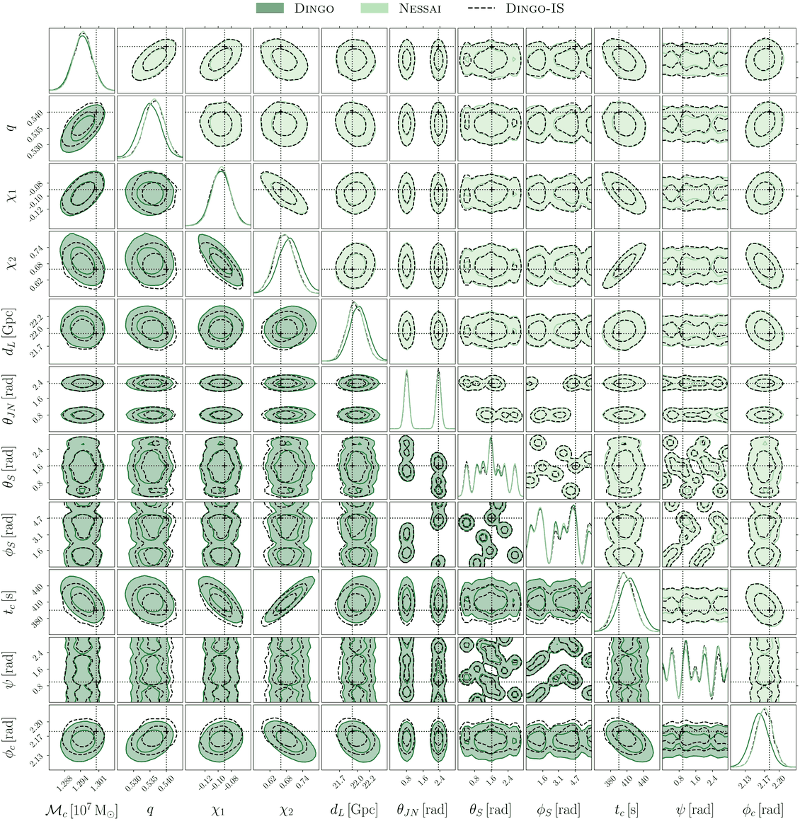
Fig. 4 — duplicated top and right axis labels cropped.
- The problem. A massive black-hole binary in the LISA band — \(\mathcal{M}_c = 1.3\times10^{7}\,M_\odot\), \(d_L = 21.9\) Gpc, SNR \(\approx 500\). Eleven parameters, and the low-frequency LISA response leaves sky position \((\theta_S,\phi_S)\) and polarisation \(\psi\) strongly multimodal.
- The architecture. DINGO's ground-based network, carried over to LISA: a conditional normalising flow of rational-quadratic spline coupling transforms, fronted by an embedding network that compresses each channel's strain into a 128-dimensional feature vector — the flow sees only those summaries.
- What it shows. The angular multimodality is reproduced almost exactly, but the raw flow (dark green) sits visibly off the nested sampler (light green) in \(q\), \(\chi_2\), \(t_c\) and \(\phi_c\). Importance sampling against the true likelihood (Dingo-IS, dashed) removes the shift, at \(\epsilon = 12\%\) efficiency — under a minute per event, against 10–40 days for the unaccelerated Nessai runs.
Spadaro et al. 2026, “Accurate and efficient simulation-based inference for massive black-hole binaries with LISA”, arXiv:2603.20431 — DINGO in the LISA band; importance-sampling correction: Dax et al. 2023, arXiv:2210.05686.
Neural SBI > III. Density estimation · Flow matching
Flow matching in three equations
Flow matching is a continuous normalising flows that is easy to train and easy to evaluate. The motion is a velocity field \(v_\phi(\theta,t)\), a plain MLP taking a position \(\theta\) and a time \(t\in[0,1]\).1. Sample. Integrate the learned field from noise to data:
2. Evaluate. Integrate backwards, accumulating the divergence:
3. Train. Learn the average velocity of straight lines from \(\theta_0\) to \(\theta_1\) crossing a specific point:
No invertibility constraint, no triangular Jacobian. Training is plain regression.
Lipman et al. 2022, arXiv:2210.02747 · Liu et al. 2022, arXiv:2209.03003 · Albergo & Vanden-Eijnden 2022, arXiv:2209.15571 · Dax et al. 2023, arXiv:2305.17161 (flow matching for SBI)
Neural SBI > III. Density estimation · Flow matching
Why random pairs give the right field
Straight lines cross, so no single pair defines the motion. Least squares averages them, and that average is exactly right.To prove. The field must satisfy the continuity equation, and then the ODE's marginals are \(p_t\), so \(\theta(1)\sim p_1=p\):
Proof. For any test function \(\varphi\):
- \(\theta_t\) is affine in \(t\), so \(\dot\theta_t=\theta_1-\theta_0\)
- \(\nabla\varphi(\theta_t)\) depends only on \(\theta_t\), so swap the arrow for its conditional mean
- \(\varphi\) arbitrary, so the equation holds pointwise
- The trajectories are not the straight lines. Those cross, ODE paths cannot
- The pairing is destroyed; only \(p_t\) survives, so the coupling need not be optimal
- Endpoints are free: \(p_0=\mathcal N(0,I)\), \(p_1=p\) by construction
Neural SBI > III. Density estimation · Flow matching
Flow matching — watch the flow
Left: what training sees. Random pairs (noise \(\theta_0\), data \(\theta_1\)) joined by a straight line; the network is asked, at the dot \(\theta_t\), to output the arrow \(\theta_1-\theta_0\). Pairs are drawn independently.
Right: what the average of those arrows does. Integrating \(d\theta/dt = v^\star(\theta,t)\) carries a Gaussian blob (t=0) onto the target (t=1).
Note: Nothing here is trained (see below).
Neural SBI > III. Density estimation · Flow matching
Aside: no network is being trained in that demo
The optimal velocity field for a finite sample set is known in closed form.
Take the straight-line interpolant and a target that is just a bag of points \(\{\theta_1^j\}\). At time \(t\), the paths starting from \(\mathcal N(0,I)\) put a Gaussian of width \((1-t)\) around each \(t\,\theta_1^j\), so the marginal is a mixture,
Given \(\theta\) and a specific endpoint \(\theta_1^j\), the noise point is pinned: \(\theta_0 = (\theta - t\,\theta_1^j)/(1-t)\), so that pair's arrow is \((\theta_1^j - \theta)/(1-t)\). The loss minimiser is the average arrow, weighted by how plausible each endpoint is:
That is what the browser evaluates, 420 particles against 420 target points, every frame. So the animation is not an approximation of flow matching: it is the field a perfectly trained network would converge to.
Neural SBI > III. Density estimation · Flow matching
Application: decomposing fast radio bursts into pulses
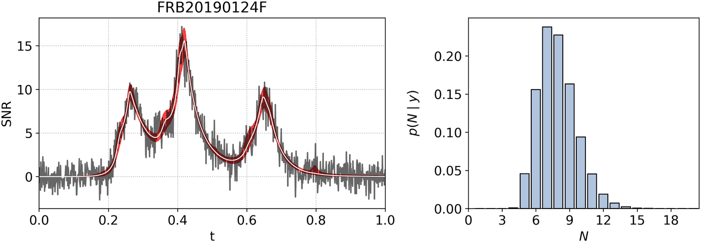
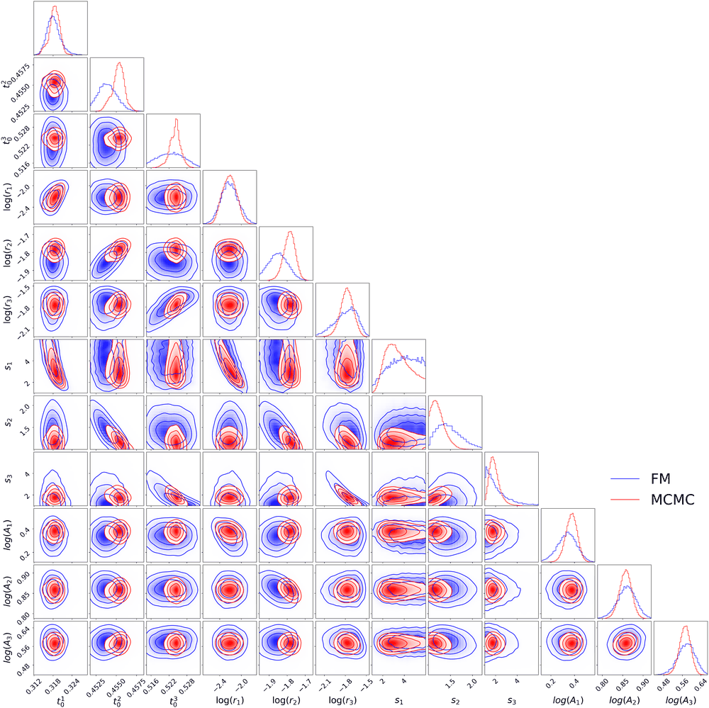
- Trans-dimensional. \(N\) is inferred, not fixed, so the parameter space has no fixed dimension: a classifier head gives \(p_\phi(N\mid y)\), and with \(N_{\max}=20\) the full \(\theta\) carries 80 entries.
- Flow matching on a transformer is the enabling combination: one token per component, masked to the \(N\) active, so a single velocity field covers every \(N\). 100 samples/s, orders of magnitude faster than MCMC.
- Not exact. Against MCMC at fixed \(N=3\) the correlations are reproduced, but the FM posterior is broader and \(t_0^2\), \(\log r_2\) are off-set (C2ST 86%) — good qualitative agreement, no more.
Left: figure 16, FRB20190124F. Right: figure 18, FRB20190115B with \(N=3\) enforced.
van der Meulen et al. 2026, Fast inference on astronomical time series with trans-dimensional flow matching posterior estimation, arXiv:2607.21134.
Neural SBI > III. Density estimation
The density-estimator zoo
Everything used as an inference head, and what each gives up.
| representation | flexible? | evaluate | sample | typical use |
|---|---|---|---|---|
| Histogram / KDE no network at all |
non-parametric | exact | resample | 1-2 D only; dies of dimensionality |
| Gaussian head network predicts \(\mu,\Sigma\) |
almost nothing | exact, instant | exact, instant | baselines, well-behaved unimodal posteriors |
| Mixture density net \(K\) weighted Gaussians |
multimodal, but \(K\) fixed | exact, instant | exact, instant | the original NPE (Papamakarios & Murray 2016) |
| Autoregressive MADE, MAF, PixelCNN |
high | exact, one pass | \(d\) sequential passes | density evaluation dominated workloads |
| Normalising flow coupling / spline layers |
architecture-limited | exact | exact | the SBI workhorse; DINGO, sbi, swyft |
| Energy-based / ratio \(q_\phi \propto e^{-E_\phi(\theta)}\) |
unrestricted | only up to \(Z\) | MCMC, slow | NRE; marginal posteriors |
| Flow matching / diffusion learn a velocity or a score |
unrestricted MLP | ODE solve | ODE / SDE solve | current best for high-D and field-level posteriors |
Row by row — mixture density net: Bishop 1994, NCRG/94/004 · autoregressive: Germain et al. 2015 (MADE), arXiv:1502.03509; Papamakarios et al. 2017 (MAF), arXiv:1705.07057 · flows: Dinh et al. 2016 (RealNVP), arXiv:1605.08803; Durkan et al. 2019 (splines), arXiv:1906.04032 · ratio: Cranmer, Pavez & Louppe 2015, arXiv:1506.02169 · continuous / score: Chen et al. 2018 (neural ODE), arXiv:1806.07366; Song et al. 2021 (score SDE), arXiv:2011.13456.
Neural SBI > IV. Summary extraction
IV. Summary extraction
The component that replaces ABC's hand-picked statistic. It is where the data type enters, and the only place information can be lost for good.
Neural SBI > IV. Summary extraction
Getting the data into the network
The recipe never changes: a stack of learned affine maps and nonlinearities, fitted by gradient descent. What changes is the wiring, chosen to match the data.
MLPCNN1D CNN, SVD + ResNetGraph NN, DeepSetsTransformerU-NetThe SVD + ResNet strain embedding is DINGO: Dax et al. 2021, arXiv:2106.12594.
Neural SBI > IV. Summary extraction
Application: embedding a 3D density field in wavelets
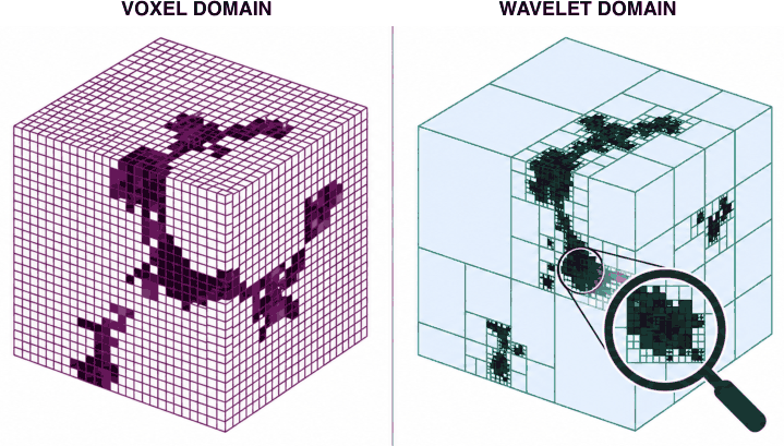
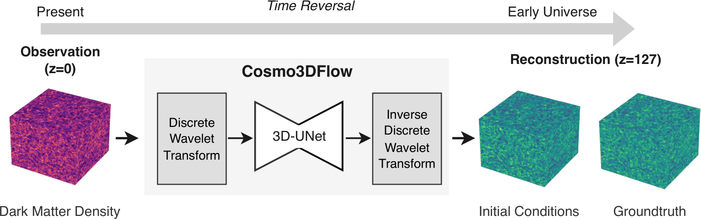
- The task. Sample the \(z=127\) initial conditions given the present-day \(z=0\) density field — the field-inference problem from earlier (Falcon + Disco-DJ at \(64^3\)), now on Quijote at \(128^3\).
- Here the first stage is deliberately not learned. One level of the 3D Haar transform reshapes \(128^3\) into eight subbands at \(64^3\), and the conditioning field enters the same way. Nothing is thresholded: voids become near-zero coefficients rather than excised, since they still carry large-scale modes.
- Lossless by construction — but the basis alone buys nothing. It is orthogonal, so nothing is lost in the embedding; it all rides on the network. And naive wavelet flow matching is worse than voxel-space (VRMSE 0.34 vs 0.26) until the U-Net is rewired with per-scale conditioning and cross-scale skips.
Left: figure 1 — sparse, scattered voxel structure becomes compact in a wavelet basis; the drawn subdivision is schematic, not the transform used. Right: figure 2, metrics panel cropped; \(\approx 5\) s/sample at \(128^3\) vs \(259\) s for diffusion.
Islam et al. 2026, Cosmo3DFlow: Wavelet Flow Matching for Spatial-to-Spectral Compression in Reconstructing the Early Universe, arXiv:2602.10172.
Neural SBI > IV. Summary extraction
Information content: the definitions
| Entropy | \[ H(X) = -\sum_x p(x)\log p(x) \] Average uncertainty in \(X\). How many bits does it take to describe a draw from \(p(x)\)? |
| Conditional Entropy | \[ H(X\mid Y) = -\sum_{x,y} p(x,y)\log p(x\mid y) \] Remaining uncertainty in \(X\) after observing \(Y\). |
| Mutual Information | \[ I(X;Y) = H(X) - H(X\mid Y) = \sum_{x,y} p(x,y)\log\frac{p(x,y)}{p(x)p(y)} \] How much knowing \(Y\) reduces uncertainty about \(X\). Zero iff \(X \perp Y\). |
Neural SBI > IV. Summary extraction
NPE learns information-maximizing summaries
Add a summary network, \(q_\phi(\theta\mid x)\to q_\phi(\theta\mid T_\phi(x))\). Then
Tight when the estimator is exact. Training \(T_\phi\) end to end pushes summaries toward minimal posterior entropy.
Using the identity
\[ \mathbb{E}_{p(x)} H\big(p(\theta\mid T_\phi(x))\big) = H\big(p(\theta)\big) - I\big(\theta; T_\phi(x)\big) \]we find that
minimizing posterior entropy \(\;\Leftrightarrow\;\) maximizing \(I(\theta; T_\phi(x))\).
Summaries learned in the context of NPE (and NRE, and score matching, but not NLE)
are information-maximizing. That is a key strength.
It also brings one of the hardest open problem in the field: knowing when they are sufficient.
Charnock, Lavaux & Wandelt 2018, arXiv:1802.03537 (IMNN: training summaries by an information criterion directly).
Neural SBI > IV. Summary extraction
Information content: a Venn diagram view
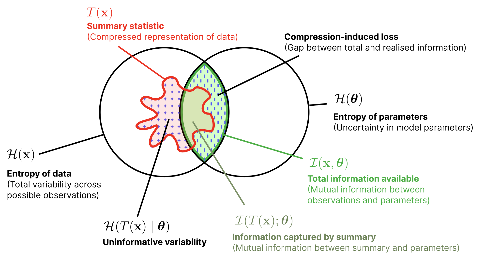
Any deterministic function \(T(x)\) can only destroy, never create, information about \(\theta\).
\[ T(x)\ \text{sufficient} \;\Leftrightarrow\; I(\theta;\,T(x)) = I(\theta;\,x) \]
Equality holds iff \(\theta \perp x \mid T(x)\): the statistic captures everything about \(\theta\).
Compressing \(x \to T(x)\) before SBI can only widen posteriors. The ideal learned summary is a sufficient statistic.
The data-processing inequality and sufficiency are standard: Cover & Thomas, Elements of Information Theory, 2nd ed., Wiley 2006, chs. 2 and 2.9.
Which one when > Information
Where does the information come from?
Both target the same posterior. They differ in what the computer is handed.
One call returns a single number: how well this \(\theta\) agrees with the data. Nothing about what went wrong, or where to look next.
Highly informative per call, so the work is exploring parameter space.
Each call returns the whole data vector, and the network sees thousands side by side. The work is extracting what is relevant.
Structure is learned rather than explored, but information can be lost on the way in.
Limited by compute in parameter space on the left, by information loss in data space on the right.
Which one when > Decision
When to use what
| Situation | Reach for | Why |
|---|---|---|
| Likelihood is exact, cheap, and \(d_\theta\) is small | MCMC / nested sampling | Nothing to gain from learning. Exact, well understood, and the diagnostics are mature. |
| Likelihood is exact but the forward model is slow | Emulator + MCMC | Learn \(\theta \mapsto\) observable, keep the likelihood. Example: CosmoPower. |
| Nuisances or latent structure make the likelihood intractable | Any SBI | Sampling a nuisance inside the simulator replaces an integral you cannot do. |
| The same analysis is repeated on many events | NPE (amortised) | Training cost is paid once; each new event is a forward pass. The DINGO regime. |
| One observation, very expensive simulator | Sequential / dynamic SBI | Amortisation is wasted effort. Spend the budget near the data. |
| The prior may change after the analysis | NRE or NLE | Both learn prior-independent objects; NPE bakes the prior in. |
CosmoPower: Spurio Mancini et al. 2021, arXiv:2106.03846 · the amortised-NPE regime: Dax et al. 2021, arXiv:2106.12594 · benchmarks behind these recommendations: Lueckmann et al. 2021, arXiv:2101.04653.