Simulation-based Inference

Lecture 2 — Diagnostics, sequential methods, and scale

Christoph Weniger — University of Amsterdam (GRAPPA)
IAIFI PhD School, 6 August 2026

Diagnostics

A learned posterior always returns something. Knowing when to believe it is a separate problem.

Diagnostics > Taxonomy

Where can inference go wrong?

A taxonomy of epistemic uncertainties in SBI: three failure modes, each with its own diagnostic strategy.

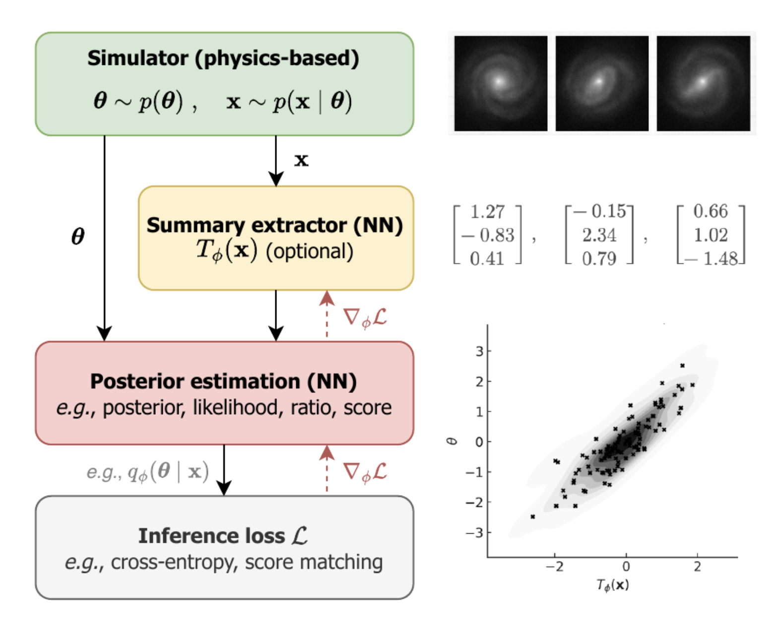
Category	Type	Description
Epistemic	Epi-R	Reality Gap "I'm simulating the wrong system"
	Epi-C	Compression Gap "I'm discarding relevant information"
	Epi-A	Approximation Gap "I can't compute the posterior exactly"
Aleatoric	Ale	Irreducible randomness in the system and data

Diagnostics > Failure modes

Overdispersion vs lossy summaries

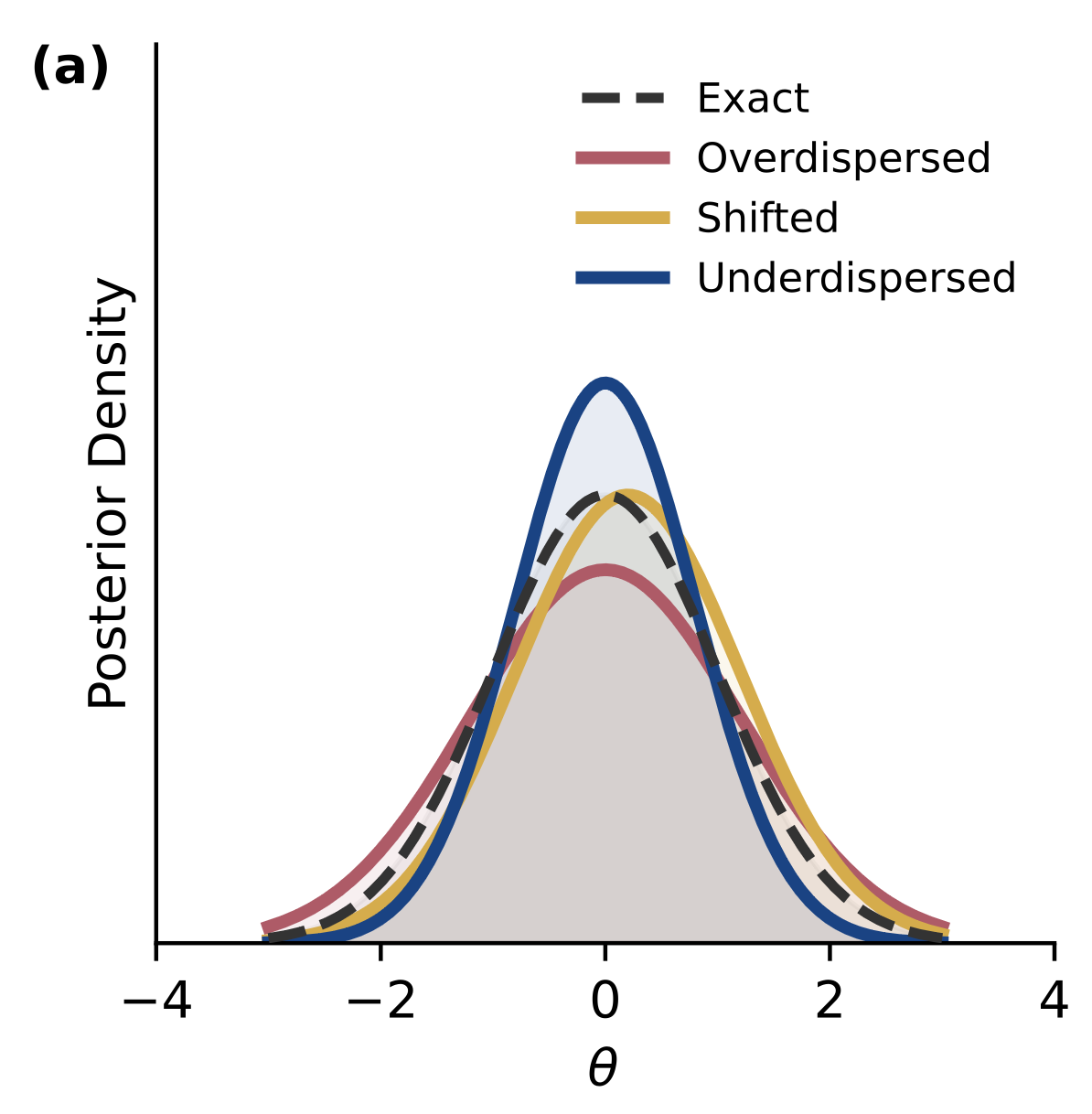
Approximate posteriors \(q_\phi(\theta \mid x)\) are overdispersed (underdispersed) when they overestimate (underestimate) their coverage of the data-generating parameters (example for Epi-A).

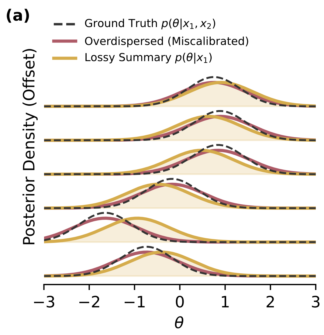
Posteriors that are exact but based on a lossy summary, \(q_\phi(\theta \mid x) = p(\theta \mid T(x))\), are wider and not overdispersed. Their width correctly represents the information loss, and the extra scatter in the posterior position exactly compensates. This is Epi-C.

Diagnostics > Reference posteriors

Comparing against a reference posterior

The most direct question you can ask: does the learned posterior agree with one we already trust?

\[ q_\phi(\boldsymbol\theta \mid \mathbf{x}_\mathrm{obs}) \;\;\overset{\text{consistent with?}}{\longleftrightarrow}\;\; p(\boldsymbol\theta \mid \mathbf{x}_\mathrm{obs}) \]

Reference may be available as unnormalised explicit posterior, through Fisher approximation, or MCMC samples, etc.

On simulated data

Epi-C shows up as a learned posterior that is broader than the reference, but centred correctly.
Epi-A shows up as bias, missing modes, or other structural distortions.

On real data

Epi-R now enters too: SBI and likelihood-based methods may respond differently when the model is wrong. A disagreement here is informative but ambiguous.

Cannon, Ward & Schmon 2022, arXiv:2209.01845 (misspecification and SBI) · review: Cranmer, Brehmer & Louppe 2020, arXiv:1911.01429.

Diagnostics > Reference posteriors

Which divergence, and what it is sensitive to

A divergence quantifies the difference between two distributions. They all vanish when \(p = q\), and they weight disagreements very differently.

\[ D_f(p \,\|\, q) = \int d\theta\; q(\theta)\, f\!\left(\frac{p(\theta)}{q(\theta)}\right) \]

Divergence	generator \(f(t)\)
KL, \(D_\mathrm{KL}(p\\|q)\)	\(t\log t\)
Neyman \(\chi^2\)	\((t-1)^2\)
Jeffreys, \(D_J(p;q)\)	\((t-1)\log t\)
Jensen-Shannon	\(\tfrac{1}{2}\!\left(t\log t - (t{+}1)\log\tfrac{t+1}{2}\right)\)
Total variation	\(\tfrac{1}{2}\|t-1\|\)

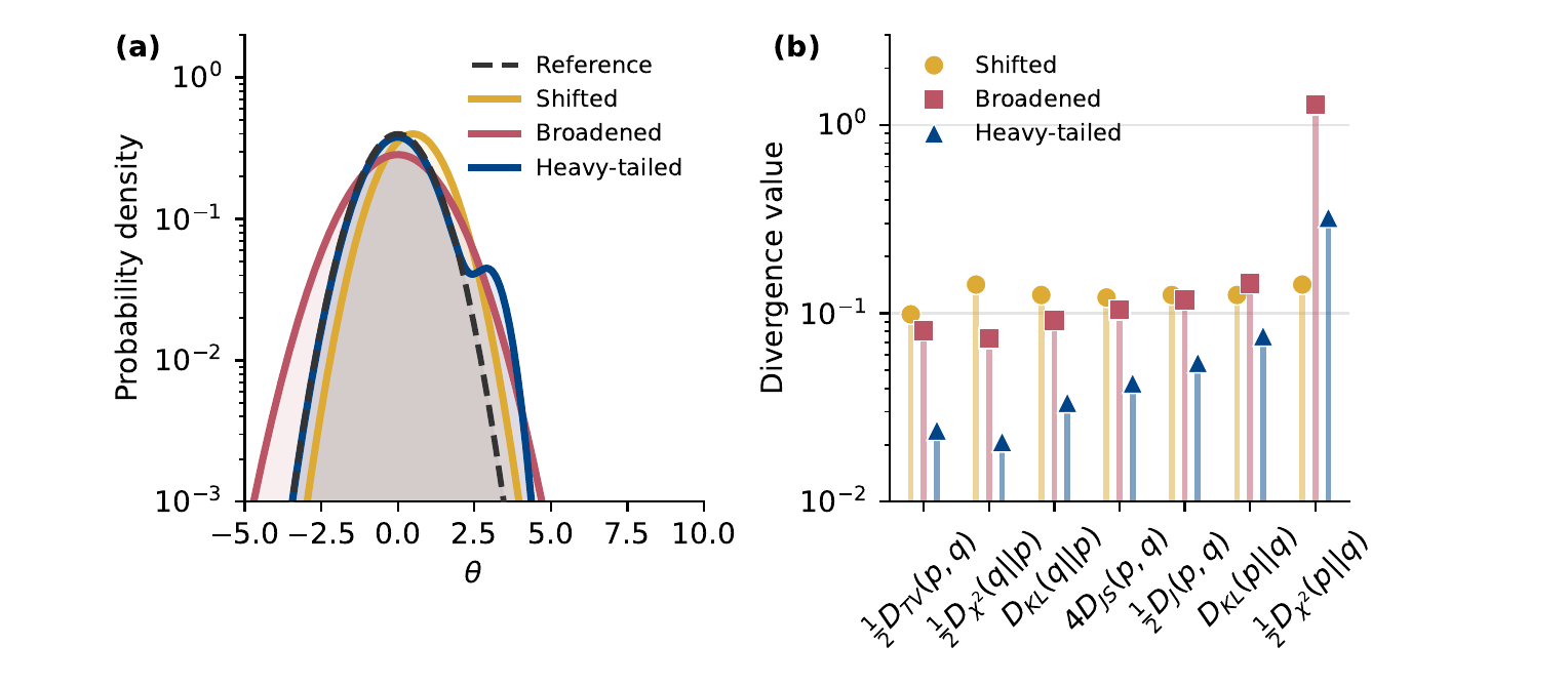
Values are rescaled by \(f''(1)\) so that a shifted posterior gives comparable numbers, and ordered by sensitivity to unmodelled modes.

Diagnostics > Reference posteriors

Estimating a divergence from samples

If the unnormalised posterior can be evaluated. With \(\pi(\theta\mid x) = p(x\mid\theta)p(\theta) = Z\,p(\theta\mid x)\), draw \(\theta_i \sim q_\phi\) and estimate the missing constant, \[ Z \simeq \frac1N \sum_i \frac{\pi(\theta_i\mid x)}{q_\phi(\theta_i\mid x)}, \qquad w_i = \frac{\pi(\theta_i\mid x)}{Z\, q_\phi(\theta_i\mid x)} . \] Any \(f\)-divergence follows from the \(w_i\).

The same weights also fix the posterior. Resample the \(\theta_i\) with probabilities \(\tilde w_i = w_i/\sum_j w_j\) and you have normalised importance sampling: an approximation to \(p(\theta\mid x_\mathrm{obs})\) that becomes exact as \(N \to \infty\), provided \(q_\phi\) covers the support of \(p\). This is what DINGO-IS does.

Effective sample size. A cheap, interpretable quality number: it saturates when \(q_\phi\) matches the target and collapses when one sample carries all the weight. \[ \mathrm{ESS} \equiv \frac{1}{\sum_i \tilde w_i^{\,2}}, \qquad 1 \le \mathrm{ESS} \le N \]

Diagnostics > Forward-backward

When there is no reference: forward-backward consistency

If no trustworthy reference posterior exists, one can use self-consistency checks: comparing joint samples from the backward model and the forward model.

\[ \underbrace{q_\phi(\boldsymbol\theta\mid\mathbf{x})\,p(\mathbf{x})}_{\text{backward (inference)}} \;\;\overset{\text{consistent with?}}{\longleftrightarrow}\;\; \underbrace{p(\mathbf{x}\mid\boldsymbol\theta)\,p(\boldsymbol\theta)}_{\text{forward (simulator)}} \]

If \(q_\phi(\boldsymbol\theta\mid\mathbf{x}) = p(\boldsymbol\theta\mid\mathbf{x})\) the two joint distributions coincide exactly. Conversely, any discrepancy is a clear indicator of inference error.

Epi-R: not detected. Both sides are generated from the same assumed model, so misspecification cancels out perfectly.

Epi-C: mostly invisible. A posterior based on a lossy summary is still a valid posterior, just a wider one. Only a few special orderings can see it.

Epi-A: the primary target. Bias, wrong width, missing modes, and most other inference errors leave a signature.

Talts et al. 2018 (SBC), arXiv:1804.06788 · Cook, Gelman & Rubin 2006, JCGS 15, 675 · Modrák et al. 2023 (what the histogram can and cannot see), arXiv:2211.02383.

Diagnostics > Forward-backward · SBC

Simulation-based calibration

Algorithm:

Draw \(\theta^*\sim p(\theta^*)\) from the prior.
Run the simulator to get \(x \sim p(x\mid\theta^*)\).
Draw \(L\) samples \(\theta_{1:L}\) from the learned posterior \(q_\phi(\theta\mid x)\).
Record the rank of \(\theta^*\) among them. \[ F(\theta^*) = \tfrac{1}{L}\sum_{i=1}^{L} \mathbb{1}(\theta_i \le \theta^*) \]
Repeat \(N\) times; histogram the ranks.

"Prior, then simulator" is the same thing as "\(x\sim p(x)\), then \(\theta^*\sim p(\theta\mid x)\)". Under \(q_\phi = p\) all \(L+1\) rank positions are equally likely, so the histogram is flat.

bias \(b\) = 0.000 scale \(s\) = 1.00

trials: 0

Simulator \(\theta\sim\mathcal{U}(-1,1)\), \(x\mid\theta\sim\mathcal{N}(\theta,\sigma^2)\) with \(\sigma = 0.1\); learned posterior \(q_\phi(\theta\mid x) = \mathcal{N}(\theta;\, x+b,\, (s\sigma)^2)\). Red × is \(\theta^*\); orange dots are the \(q\)-samples whose rank we record.

Diagnostics > Forward-backward · Coverage

Highest-posterior coverage tests

Algorithm:

Draw \(\theta^*\sim p(\theta^*)\) from the prior.
Run the simulator to get \(x \sim p(x\mid\theta^*)\).
Draw \(L\) samples \(\theta_{1:L}\) from the learned posterior \(q_\phi(\theta\mid x)\).
Record the rank of \(\theta^*\) among them. \[ F(\theta^*) = \tfrac{1}{L}\sum_{i=1}^{L} \mathbb{1}(q_i \ge q^*) \]
Repeat \(N\) times; histogram the ranks.

Only step 4 differs from SBC: rank by density \(q_i \equiv q_\phi(\theta_i\mid x)\), not by value. Flat now means correct highest-posterior-density coverage.

bias \(b\) = 0.000 scale \(s\) = 1.00

trials: 0

The dots now sit on the orange curve at their density height, and horizontal lines carry those heights to the axis. The red line marks \(q_\phi(\theta^*\mid x)\); the rank counts the orange lines above it.

The expected-coverage test and the "conservative vs overconfident" reading: Hermans et al. 2021, arXiv:2110.06581.

Diagnostics > Failure modes

Three ways these tests go blind

A flat rank histogram is necessary, not sufficient. Three distinct failures survive it, and each has a different fix.

Averaging hides local bias. SBC integrates over \(x \sim p(x)\). A bias whose sign flips across data space partially cancels, so the global histogram can look nearly flat while calibration is badly violated in specific regions.
Fix: stratify by anything the miscalibration might depend on, signal-to-noise, sky location, observing run. The cost is statistical power per stratum.

Information loss is not miscalibration. A posterior computed from a lossy summary \(T(x)\) is a perfectly valid posterior, just a wider one. Every forward-backward test is designed to pass it. This is Epi-C, and it is invisible by construction.
Fix: an ordering function that uses the model, such as the likelihood or the score, rather than only the learned posterior.

Coverage only checks mass, not shape. HPDR tests ask how much probability lies inside a super-level set. A distortion that preserves mass-against-level, even one that turns a unimodal posterior into a bimodal one, leaves the pp-plot perfectly diagonal.
Fix: combine orderings. HPDR, central interval, one-sided limits and plain SBC each close a different blind direction.

Diagnostics > Failure modes

Each test has a whole family of blind spots

Each tests probes the contained mass of superlevel sets defined by the ordering function. Tests are blind to mass transport along the fibers of the ordering function.

Example\(^\ast\):

shift magnitude = 1.20

\(^\ast\)Construct \(q(\theta) = g(|\theta - \theta_0|)\) so that every symmetric interval around \(\theta_0\) carries exactly the true posterior mass. Then the HPDR pp-plot is diagonal by construction, no matter how distorted the shape becomes.

Lesson: combine rank-based tests. Each closes another blind direction.

Diagnostics > Failure modes

Overdispersed, or just lossy?

Algorithm:

Draw \(\theta^*\sim p(\theta^*)\) from the prior.
Run the simulator to get \(x_1, x_2 \sim p(x\mid\theta^*)\).
Draw \(L\) samples \(\theta_{1:L}\) from the learned posterior \(q_\phi(\theta\mid x)\).
Record the rank of \(\theta^*\) under the ordering \(f\): \[ F(\theta^*) = \tfrac{1}{L}\sum_{i=1}^{L} \mathbb{1}\bigl(f(\theta_i) \ge f(\theta^*)\bigr) \]
Repeat \(N\) times; histogram the ranks.

Two observations, so \(p(\theta\mid x_1,x_2)=\mathcal{N}\bigl(\tfrac{x_1+x_2}{2},\tfrac{\sigma^2}{2}\bigr)\). Both \(q\) are wider than that. Only an ordering that reads the full data sees the lossy one.

rank by \(s\) = 1.40

trials: 0

Overdispersed (width \(s\,\sigma/\sqrt2\)): every ordering sees it. Lossy (exact given \(x_1\) alone): only \(p(x\mid\theta)\) sees it.

Diagnostics > Generalization

Generalized rank diagnostics: one framework

All forward-backward tests share a structure: choose an ordering function \(f(\boldsymbol\theta, x)\) and rank \(\theta^*\) among the \(\theta_{1:L}\) under that ordering.

Method	Ranks by	Tests Epi-C	Ordering \(f(\boldsymbol\theta, x)\)
SBC	parameter (\(d\) tests)	No	\(\theta_i\) for \(i=1,\ldots,d\)
HPDR coverage	learned posterior	No	\(q_\phi(\boldsymbol\theta\mid x)\)
TARP	distance to reference	No/Yes	\(\\|\boldsymbol\theta - \boldsymbol\theta'\\|^2\)
Likelihood ranks	likelihood	Yes	\(p(x\mid\boldsymbol\theta)\)
True HPDR	true posterior	Yes	\(\pi(\boldsymbol\theta\mid x) \propto p(x\mid\boldsymbol\theta)p(\boldsymbol\theta)\)

Completeness: If the rank statistic is uniform for every ordering \(f(\boldsymbol\theta, x)\), then \(q_\phi = p\) almost everywhere (Lemos et al. 2023). Any finite set of orderings is necessary but not sufficient.

Lemos et al. 2023 (TARP), arXiv:2302.03026 · Modrák et al. 2023 (the choice of test quantity shapes sensitivity), arXiv:2211.02383.

Diagnostics > Misspecification

Model Misspecification (Epi-R): two starting points

Two separable questions about the simulator, joined by a named deviation of amplitude \(\eta\).

\(p(\mathbf{x}\mid\boldsymbol\theta)\) — baseline simulator.

\(p_\eta(\mathbf{x}\mid\boldsymbol\theta)\) — augmented simulator: consider one named deviation, amplitude \(\eta\), with \(p_{\eta=0} = p\).

\(p^*(\mathbf{x}\mid\boldsymbol\theta)\) — the real data generating process; typically never sampled.

Step 1 · data space

"Is there an indication of a deviation?"

\[ H_0:\ \mathbf{x}\sim p(\mathbf{x}\mid\boldsymbol\theta) \quad\text{vs.}\quad H_\eta:\ \mathbf{x}\sim p_\eta(\mathbf{x}\mid\boldsymbol\theta) \]

Test statistic: discriminator between \(p\) and \(p_\eta\).
Null from simulation: one observation suffices.
Detections or exclusions on \(\eta\).

Step 2 · parameter space: Why would it matter?

\[ \mathop{\mathbb{P}}\limits_{\substack{\theta^*\sim p(\boldsymbol\theta)\\ \mathbf{x}\sim p_\eta(\cdot\mid\theta^*)}} \bigl[\,\theta^*\in\mathrm{HPD}_\alpha\bigl(q_\phi(\cdot\mid\mathbf{x})\bigr)\,\bigr] \;\overset{?}{=}\;\alpha \]

\(q_\phi\) frozen: trained on \(p\), evaluated on \(p_\eta\). No retraining.
Same coverage test, different simulator.

Step 1 ↓ Step 2 →	inference insensitive	inference sensitive
no deviation found	fine, and you can say why	the dangerous cell
deviation found	model wrong, but it doesn't matter	fix the simulator

Some literature on misspecification in SBI: Cannon, Ward & Schmon 2022, arXiv:2209.01845 · Ward et al. 2022 (robust SBI), arXiv:2209.11057 · posterior predictive checks: Gelman, Meng & Stern 1996, Statist. Sinica 6, 733.

Diagnostics > Misspecification

Hypothesis testing at volume

SBI enables the massively parallelize hypothesis testing to search for localized or aggregated devitations in data.

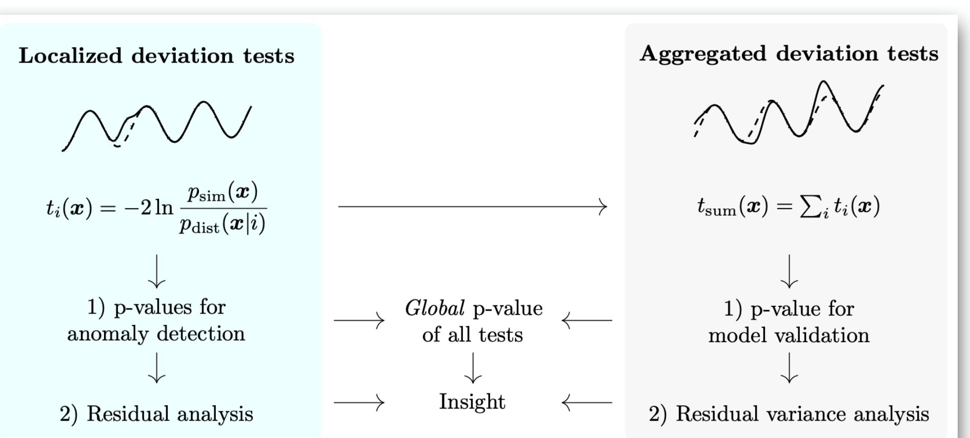
Network training is cheap, enabling a broad battery of tests to probe many forms of distortion.
Provides p-values for both local anomalies and global goodness-of-fit, offering structured diagnostics.
Method is ready for real data, illustrated here on the landmark GW150914 event.

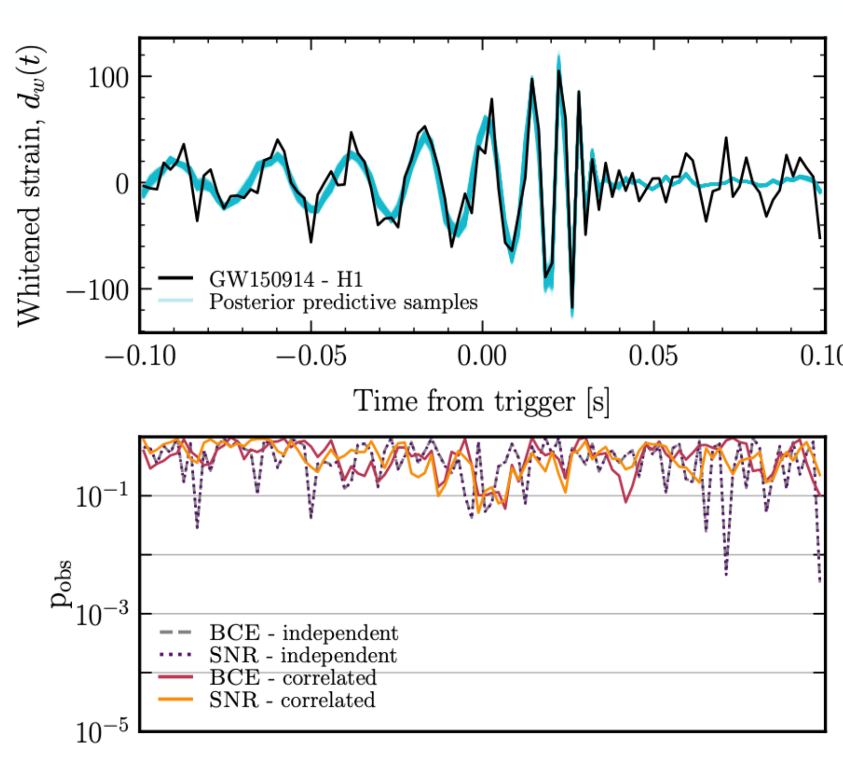
Noemi Anau Montel (MPA) · Anau Montel, Alvey & Weniger 2024, arXiv:2412.15100

Sequential methods

Amortisation is a luxury. When you only have one observation, stop paying for it.

Sequential methods > SNPE

Sequential neural posterior estimation

Amortised NPE spends its whole simulation budget covering the prior, so that any observation can be answered. If there is only one \(\mathbf{x}_\mathrm{obs}\), almost all of that budget is spent on data you will never see.

Strategy

Run NPE on a small number of simulations from the prior.
Update the proposal based on the learned posterior.
Repeat until the proposal is concentrated around \(\mathbf{x}_\mathrm{obs}\).

# Sequential NPE, R rounds of N simulations p̃₁ ← p(θ) # round 1 proposes from the prior D ← {} for r = 1 .. R: # 1. simulate from the current proposal for n = 1 .. N: θₙ ~ p̃ᵣ(θ) xₙ ~ p(x | θₙ) D ← D ∪ {(θₙ, xₙ)} # 2. train the head on everything seen so far φ ← argmin −∑ log qφ(θₙ | xₙ) over D # plus a correction, see next slide # 3. re-focus the proposal on the observation p̃ᵣ₊₁(θ) ← qφ(θ | x_obs) return qφ(θ | x_obs)

Papamakarios & Murray 2016, arXiv:1605.06376 · Lueckmann et al. 2017, arXiv:1711.01861 · Greenberg, Nonnenmacher & Macke 2019, arXiv:1905.07488 · Deistler, Goncalves & Macke 2022, arXiv:2210.04815.

Sequential methods > The proposal problem

A proposal is not a prior

Train on pairs drawn from \(\tilde p(\boldsymbol\theta)\,p(\mathbf{x}\mid\boldsymbol\theta)\) and the NLL minimiser is not the posterior any more. It is the proposal posterior:

\[ \tilde p(\boldsymbol\theta\mid\mathbf{x}) \;=\; p(\boldsymbol\theta\mid\mathbf{x})\; \frac{\tilde p(\boldsymbol\theta)}{p(\boldsymbol\theta)}\; \frac{p(\mathbf{x})}{\tilde p(\mathbf{x})} \]

Four families of fixes, and they differ mainly in where the correction is applied.

Correct afterwards (SNPE-A). Train normall, then divide the learned density by the ratio \(\tilde p/p\) analytically. Requires MCMC run afterwards.
Correct in the loss (SNPE-B). Keep the target as the true posterior and reweight each training pair by importance weights \(w_n = p(\boldsymbol\theta_n)/\tilde p(\boldsymbol\theta_n)\).
Correct in the model (SNPE-C). Parameterise the proposal posterior instead, as \(\tilde q_{\phi}(\boldsymbol\theta\mid\mathbf{x}) \propto q_\phi(\boldsymbol\theta\mid\mathbf{x})\, \tilde p(\boldsymbol\theta)/p(\boldsymbol\theta)\), and normalise it on an atomic set of \(\theta\) drawn from the batch.
Avoid the problem (Truncation). Do not reshape the prior, cut it. Restrict to a region that contains almost all the posterior mass and set the proposal to the prior restricted there.

Papamakarios & Murray 2016 (A), arXiv:1605.06376 · Lueckmann et al. 2017 (B), arXiv:1711.01861 · Greenberg et al. 2019 (C / APT), arXiv:1905.07488 · Miller et al. 2021 (truncated marginal), arXiv:2107.01214 · Deistler et al. 2022 (truncated SNPE), arXiv:2210.04815.

Sequential methods > Prior independence

Or: learn something the prior cannot spoil

The correction problem exists only because NPE learns \(q_\phi(\boldsymbol\theta\mid\mathbf{x})\), an object that contains the prior. Target something that does not, and sequential training needs no correction whatsoever.

Sequential NLE

The likelihood \(p(\mathbf{x}\mid\boldsymbol\theta)\) is a property of the simulator alone. Where you choose to draw the \(\boldsymbol\theta\) changes only which region gets fitted well, never what the correct answer is.

\[ \mathcal{L} = -\tfrac{1}{N}\sum_n \log q_\phi(\mathbf{x}_n\mid\boldsymbol\theta_n), \qquad \boldsymbol\theta_n \sim \tilde p \ \text{(anything)} \]

Sample the posterior at the end with MCMC on \(q_\phi \, p(\boldsymbol\theta)\), using the real prior.

Sequential NRE

The likelihood-to-evidence ratio is likewise prior-free. Train the classifier on proposal-drawn pairs, then apply the ratio to whichever prior you actually want:

\[ p(\boldsymbol\theta\mid\mathbf{x}) \;\propto\; r_\phi(\boldsymbol\theta,\mathbf{x})\,p(\boldsymbol\theta) \]

Combined with truncation this is TMNRE: cut the prior box round by round, train marginals directly, no reweighting anywhere.

The trade. NPE gives you samples in one forward pass but bakes in the prior and needs a correction the moment you go sequential. NLE and NRE stay prior-free and compose cleanly with sequential schemes, at the cost of an MCMC run per observation.

Papamakarios, Sterratt & Murray 2019 (SNL), arXiv:1805.07226 · Hermans, Begy & Louppe 2020 (SNRE), arXiv:1903.04057 · Miller et al. 2021 (TMNRE), arXiv:2107.01214.

Sequential methods > Truncation

Rounds in action — and where they stop

Fixed budget of 400 simulations per round, drawn from the prior restricted to the current box — the proposal is a cut, not a fitted density. Learn \(q_\phi(\boldsymbol\theta\mid\mathbf{x}_\mathrm{obs})\), truncate to its \(3\sigma\) marginals, repeat.

round	1
box (θ₁ × θ₂)	12.0 × 12.0
volume vs prior	1
sample spacing Δ	0.54
Δ / σ_post	3.1

box width vs round

The prior box is far wider than the posterior: almost every simulation lands where \(\mathbf{x}_\mathrm{obs}\) could never have come from.

Parameter space — fixed to the prior range

Data space — fixed axes

Truncation stalls at the information floor — the exact posterior's own \(3\sigma\) width, set by the measurement noise. There \(\Delta\) has dropped below \(\sigma_\mathrm{post}\) and the surviving models differ by less than that noise. There is nothing left to cut.

Illustration only: \(q_\phi\) here is the exact posterior blurred by the sample spacing \(\Delta\propto\sqrt{V_\mathrm{box}/N}\), standing in for a network that cannot resolve structure finer than the gaps between its training points. No network is trained.

Miller et al. 2021 (TMNRE), arXiv:2107.01214 · Deistler, Goncalves & Macke 2022 (truncated SNPE), arXiv:2210.04815.

Sequential methods > EMRIs

Cornering an EMRI — not yet a posterior

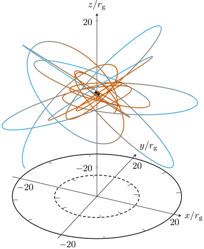
Three-dimensional view of a precessing Kerr orbit

The problem. A stellar-mass object spiralling through \(10^4\)–\(10^5\) strong-field orbits of a \(10^4\)–\(10^7\,M_\odot\) black hole: long, harmonic-rich, GPU-expensive waveforms over a vast, multi-modal 11-D space.
The scheme. TMNRE, as on the previous slide: six rounds of \(1.5\times10^5\) waveform + LISA-response simulations, \(\sim\)14 h per round on one A100, cutting each marginal prior where the ratio drops below \(10^{-5}\).

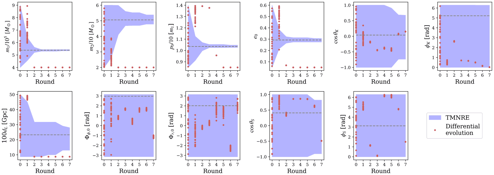
Per-round TMNRE bounds for all eleven EMRI parameters, against differential evolution

Top left: the 3-D panel of figure 1 of Berry et al. 2019. Below: figure 3 of Cole et al. 2026, its 11 panels re-tiled 6×2 here.

Cole et al. 2026 (sequential SBI for EMRIs), Phys. Rev. D 113, 063030, arXiv:2505.16795 · Berry et al. 2019 (the EMRI science case), arXiv:1903.03686.

Falcon*

Tackling complex analysis problems: many sources, many parameters, one continuous inference.

*github.com/cweniger/falcon

Falcon > Motivation

Sufficiently realistic simulation models are DAGs

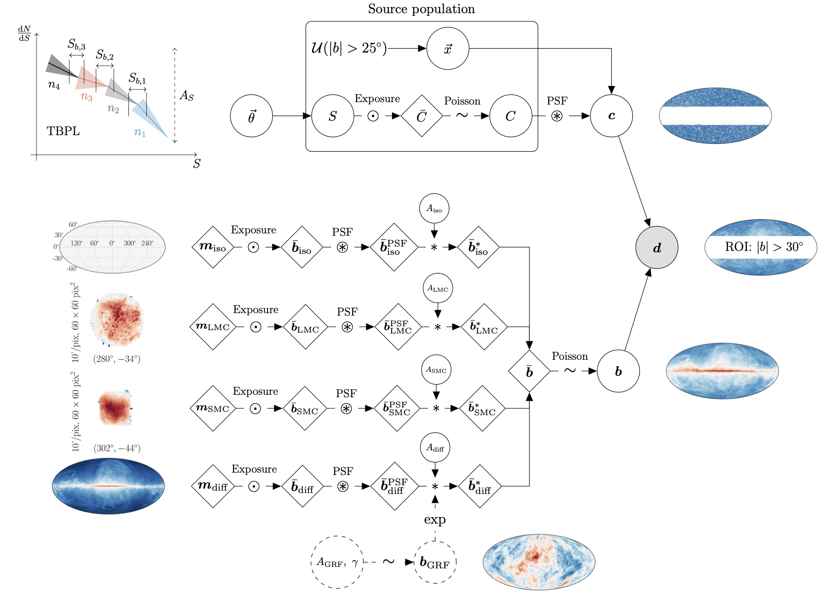
Gamma-ray astronomy

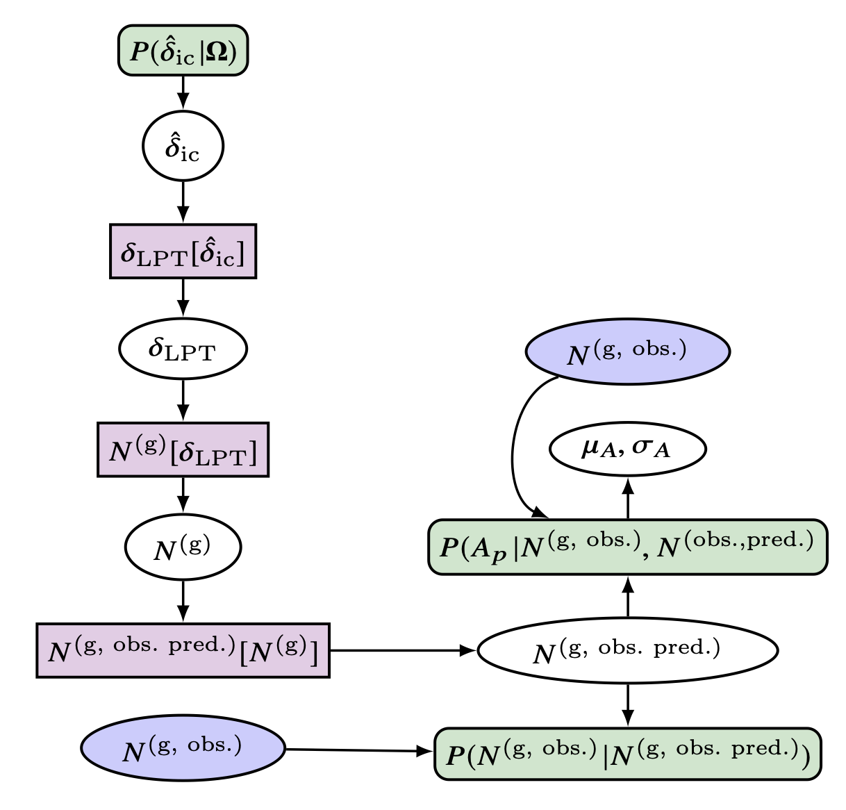
Cosmology

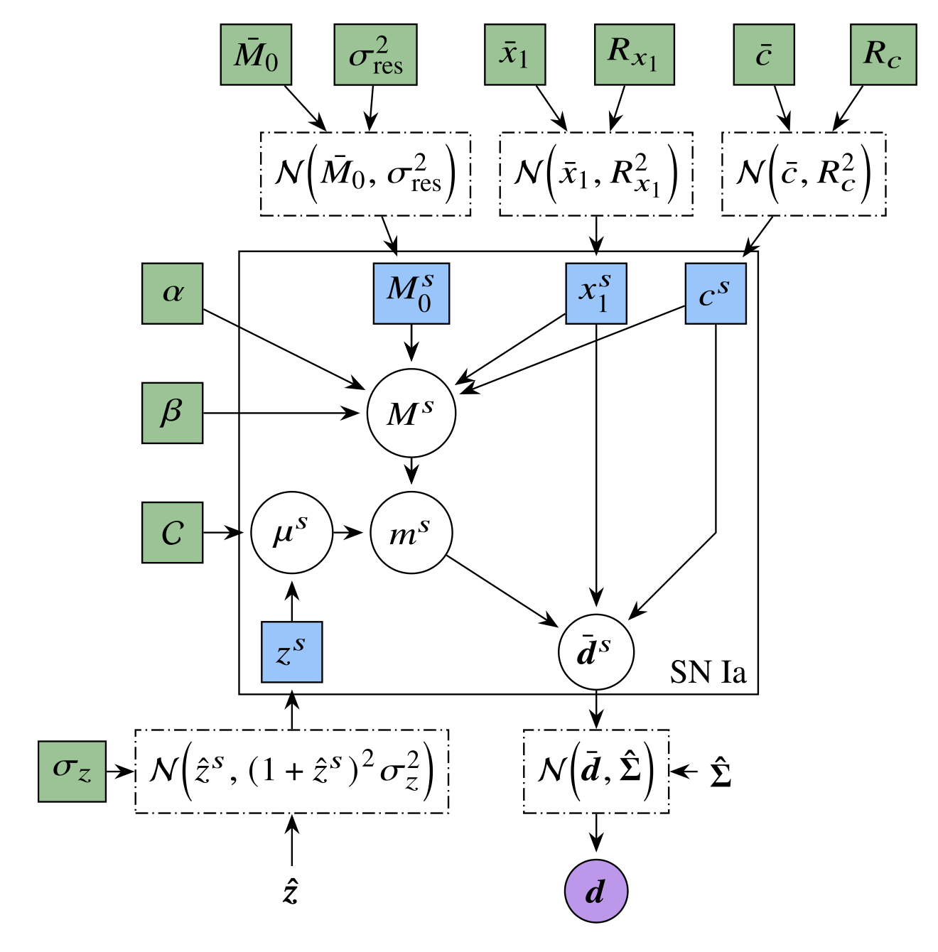
Supernova cosmology

The high-latitude gamma-ray sky as seen by Fermi-LAT — Eckner et al. (2025), arXiv:2505.02906
The cosmic matter density field behind SDSS-III/BOSS, from BORG — Lavaux et al. (2019), arXiv:1909.06396
A population of Type Ia supernovae as standard candles — Karchev et al. (2022), arXiv:2209.06733

There is no single \(\boldsymbol\theta\). Each model is a graph of many parameter components — different size, different shape, different form.

Falcon > Architecture

How Falcon is put together

1 · Declare

Complex models defined declaratively, in YAML config files.

2 · Distribute

Every component becomes its own Ray actor, spread over whatever hardware there is.

3 · Collect

All simulation data goes into one central, shared store.

4 · Close the loop

The store feeds inference actors that learn the posteriors — and steer which simulations run next.

Falcon > Dynamic SBI

Dropping the rounds — faster, same posterior

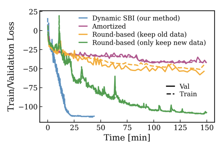
10D benchmark: loss vs. wall clock

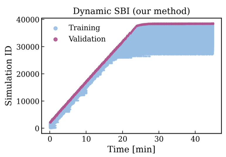
same run: which simulations sit in the training set, over time

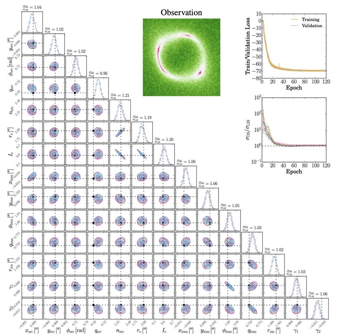
strong lensing, 14 parameters — Dynamic SBI (pink) vs. likelihood-based reference (blue)

Lyu et al. 2025 (Dynamic SBI), arXiv:2510.13997 — left: 10D benchmark (Fig. 3); right: strong lensing (Fig. 5).

Falcon > Status

It works — and it is being used

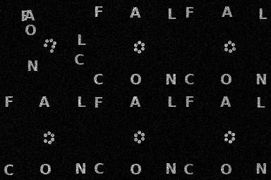
click to replay

The animation is this example's own run. Two independent latent components — a snake and the FALCON letters — each rendered, then composited into one noisy image. Both inference actors see only \(x\), and each steers what its own branch simulates next — the round-by-round contraction the animation shows. github.com/cweniger/falcon → examples/03_composite

Current application domains:

Radio interferometry: Joined reconstruction of radio images and antenna calibrations
Cosmology: Sequential SBI reconstruction of cosmological fields.
Gravitational waves — see the next slide

Falcon > LISA

A massive black-hole binary, from the full prior PRELIMINARY

LDC1-1, sequential SBI started from the full LDC prior: all-sky, ±half a day in \(t_c\), signed spins. No narrowed prior, no template bank.

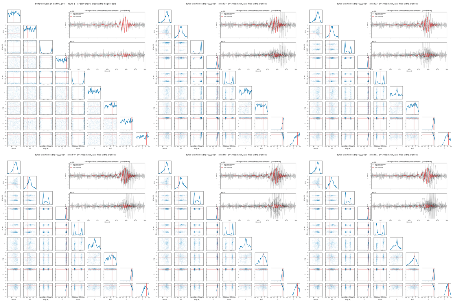
training buffer, round by round

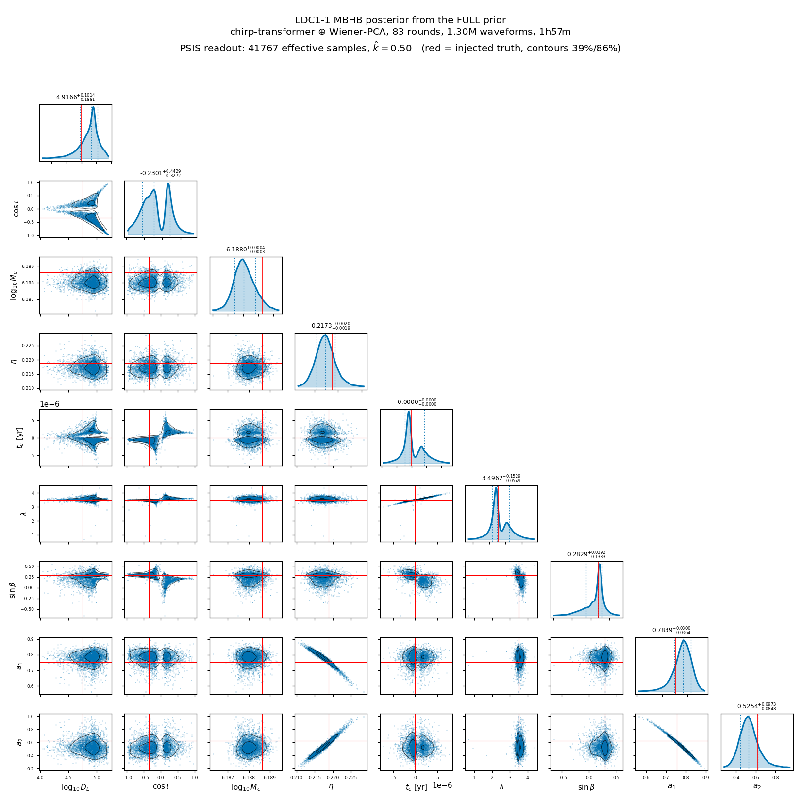
final posterior (red = injected truth)

83 rounds · 1.30M waveforms · 1 h 57 m on one GPU · 8 of 9 parameters within 1σ

H. Lyu et al., in prep. — LISA global-fit effort

Falcon > Open questions

Open questions

Composition. Which conditional independencies are assumed and which are actually learned — and do the pieces compose into a consistent joint, or only into a set of plausible marginals?
Diagnostics. Do the rank-based tests of Section 1 still apply — to each piece and to the composition?
Scaling. How does cost grow with the number of overlapping sources, at a simulation budget matched against parallel-tempered MCMC (PTMCMC), the established global-fit baseline?
Orchestration. What is worth simulating next, and how much idle time does dropping the rounds actually buy?
Robustness. Misspecification and outliers, where the diagnostics are weakest.
From bespoke to standard. Dynamic and distributed SBI as tools, not a new pipeline per analysis.

All of these are open, progress is challenging, any new insights help. Let's talk if you are interested in related problems!

Thank you!